FAST ALGORITHMS FOR SHORTEST PATHS IN PLANAR GRAPHS WITH
1 T DESIGN AND ANALYSIS OF ALGORITHMS HOMEWORK 312 SURVEYS OF THE METHODS AND ALGORITHMS FOR CALCULATING
25E COPYRIGHT 1995UNIVERSAL ALGORITHMS INCORPORATEDJULY 20 1998
4 Cs101 Algorithms and Programming i Assignment no 1
95771 DATA STRUCTURES AND ALGORITHMS FOR INFORMATION PROCESSING CARNEGIE
ADVANCED ALGORITHMS – QUIZ 3 CSE 5311 SECTION 002
FAST ALGORITHMS FOR SHORTEST PATHS
FAST ALGORITHMS FOR SHORTEST PATHS
IN PLANAR GRAPHS, WITH APPLICATIONS
GREG N. FREDERICKSON
Reporter: Bo Tian (#278636)
Background
We know that for single source problem Dijkstra's algorithm takes O(n2) time. An implementation of Dijkstra's algorithm that uses a heap improves this to O(n log n) time. Dijkstra's algorithm appeared in 1959. After 25 years later, Frederickson presented a fast algorithm in this paper that takes O(n sqrt(log n)) time. This is the first one that can beat Dijkstra’s algorithm in 25 years. Following his thoughts, people can improve the algorithm much better. This paper is very important in applied graph theory.
A number of shortest path and related problems in planar graph are presented in this paper. They are all based on the single source problem. I will give detailed description on the algorithm for single source problem.
Basic idea
The main idea in this algorithm is using r-division to divide the graph to regions, then conduct Dijkstra's algorithm on a carefully selected subset of the graph.
What is r-division
An r-division is a division into (n/r) regions of O( r ) vertices each and O(sqrt( r )) boundary vertices each.
A suitable r-division is an r-division such that:
each boundary vertex is contained in at most three regions, and
any region that is not connected consists of connected components, all of which share boundary vertices with exactly the same set of either one or two connected regions.
THEOREM 1. A planar graph of n vertices can be divided into a suitable r-division in O(n log n ) time.
Proof: Using a linear-time algorithm of Lipton and Tarjan’s Separator Theorem in Planar Graph to divide the graph recursively until we get regions at most r vertices and c*sqrt(r) (c is a constant) boundary vertices. Using methods from this paper to make sure we got a suitable r-division. The running time is O(n log n). After that we may get more regions than (n/r). We have to combine some small region that has at most r/2 vertices and at most c*sqrt( r )/2 boundary vertices to make sure there are (n/r) regions in the division. The running time is O(n). Thus the total running time is O(n log n ).
Quick way to find a suitable r-division
The paper gives a way to find a suitable r-division in O(n log r + (n/sqrt( r )) log n ) time.
Steps to find suitable r-division quickly:
Find a spanning tree of the graph using depth-first search;
Generate connected sets of (sqrt( r )) vertices in a bottom-up fashion, using a procedure FIDCLUSTERS from Data structures for on-line updating of minimum spanning trees, with applications;
Shrink the graph on these sets, yielding a planar graph Gs with (n/sqrt( r )) vertices;
Find suitable r-division in Gs with ( n/ r3/2 ) regions of cardinality O( r );
Expand Gs back to G. In G there will be O(n/r) regions of size O(sqrt( r )) resulting from boundary vertices in Gs, plus ( n/ r3/2 ) regions of cardinality O( r3/2 ) resulting from the interior vertices of Gs.
Infer boundary vertices and slightly expanded regions that share these vertices. Apply procedure that to find suitable r-division on the regions to generate a suitable r-division in G.
The running time is O(n log r + (n/sqrt( r )) log n ), since:
Step 1, 2, and 3 are O(n);
Step 4 is O(n( log n )/sqrt( r )), since there are (n/sqrt( r )) vertices in Gs;
Step 5 is O(n);
Step 6 is O(n log r ), since the region size is O( r3/2).
Procedure of the algorithm
There are two phases in this algorithm:
preprocessing phase;
search phase.
3.1 Preprocessing phase
Purpose:
To identify a subset of vertices;
To determine shortest paths between all pairs of vertices in this subset.
Use 2 level r-division to achieve the purpose.
3.1.1 Transforming
Before any other preprocessing, an original need to be transformed into a planar graph with no vertex having degree greater than 3. Using a cycle to replace a vertex having degree greater than 3. The number of vertices in this cycle is the degree of the original vertex. Each edge in this cycle has zero weight. Replace the original vertex in incident edges with respective vertex in the cycle.
3.1.2 Find r1-division
In preprocessing phase, first find a suitable r1-division of the graph, where r1 = log n. Using method described before, this step can be done in O(n log r1 + (n/sqrt( r1 )) log n ) time, which is O(n sqrt(log n)).
3.1.3 Find r2-division
For each level 1 region find a suitable r2-division , where r2 = (log log n)2. When finding this division, start with each level 1 boundary vertex automatically being a level 2 boundary vertex. This will not cause more than ( n/ sqrt( r2 )) boundary vertices of level 2 regions to be created.
This step can be done in O(r1 log r1 ) time, since the size of each region is O(r1). Then for total number of ( n/ r1 ) level 1 regions the total running time is O(n log log n).
3.1.4 Find the shortest paths between level 2 boundary vertices
For each level 2 region apply Dijkstra’s algorithm to find the shortest paths between every pair of its boundary vertices. To find a shortest path tree in one level 2 region Dijkastra’s algorithm will run in O(r2 log r2) time. Then for total number of O(n/sqrt(r2)) boundary vertices of level 2 regions the total running time is O(n log log n log log log n).
3.1.5 Find the shortest paths between level 1 boundary vertices
For each level 1 region, find the shortest paths between every pair of its boundary vertices.
This step will be done with the help of a topology-based heap. This heap is represented by a balanced tree in which the values associated with the boundary vertices appear in the leaves, with values from any one boundary set being in consecutive leaves. Whenever some vertex is closed, each region containing the vertex will have a batched update performed for each of its boundary sets. To perform a batched update, do the following. Modify the values at all leaves corresponding to vertices in the boundary set. Then proceed to modify the ancestors of these leaves level by level moving upward: first parents of the leaves, then grandparents, etc., until the value at the root is modified. The author call this procedure main thrust.
THEOREM 2. Let an n-vertex planar graph be divided into a suitable r-division. Using the associated topology-based heap, the main thrust of our algorithm will perform a set of batched update operations which cost O(n + (n/sqrt( r )) log n ).
Proof. Since there are at most O(sqrt( r )) boundary vertices per region, and each boundary set is in at most three regions, each boundary set can have a batched update performed on it at most O(sqrt( r )) times. Thus the total work involved in all batched updates for any one boundary set is proportional to sqrt( r ) log n plus sqrt( r ) times the cardinality of the boundary set. Since there are ( n/ r ) boundary sets, the total cost of the first term over all boundary sets in O((n/sqrt( r )) log n ). Since there are O(n/sqrt( r )) boundary vertices, the total cost of the second term over all boundary sets is O(n).
By using main thrust, this step can be done in O(r1 + (r1/ sqrt( r2 )) log r1), or O(r1). Then for total number of O(n/sqrt(r1)) level 1 boundary vertices, the running time is O(n/sqrt( r1 )), or O(n sqrt(log n)).
3.1.6 Total running time in preprocessing phase
O(n sqrt(log n)) + O(n log log n) + O(n log log n log log log n) + O(n sqrt(log n))
= O(n sqrt(log n))
3.2 Search phase
Two steps in search phase:
Main thrust
Mop-up
3.2.1 Main thrust
Use main thrust again. But this time apply it to the graph to find a shortest path tree encoding the shortest paths to each level 1 boundary vertex in the graph.
This time the running time is O(n + (n/sqrt( r1 )) log n ), or O(n sqrt( log n )).
3.2.2 Mop-up
Label boundary vertices with the shortest distances that got from last step to them. Apply Dijkstra’s algorithm within each region to get all shortest distances from the source.
For each r1 region Dijkstra’s algorithm will run in O(r1 log r1) time, then for total number of ( n/ r1 ) regions, this step will run in O(n log log n) time.
3.2.3 Total running time in search phase
O(n sqrt( log n )) + O(n log log n) = O(n sqrt( log n ))
Complexity of this algorithm
According to result we got before, the total running time is:
O(n sqrt(log n)) + O(n sqrt( log n )) = O(n sqrt( log n ))
Applications
Minimum cut and maximum flow
Multicommodity flows
ALGORITHMS ACTIVITY 1 LEARNER SHEET A YOU
ALGORITHMS (100199) MODEL CELL COUNT NOMINAL V V4
ALGORITHMS AND PROGRAMMING TECHNIQUES INTRODUCTION TO PROGRAM DEVELOPMENT
Tags: algorithms for, algorithms, planar, graphs, shortest, paths
- OBRAZEC ŠT 104 IZJAVA DELOVNEGA MENTORJA1 PRILOGA K VLOGI
- MECANISMO EXPERIMENTAL DE EVALUACION Y ACREDITACION INSTITUCIONAL FORMULARIO
- KOBIETA ŻYJĄCA Z HIV DR N MED TOMASZ NIEMIEC
- NR WNIOSKU DZP …………………………………………… UMOWA ZLECENIA (O ŚWIADCZENIE
- 9 JUAN J GARCÍA PELLICER JOSÉ V GARCÍA JIMÉNEZ
- SAIZAR HOTELAK KATEAREN ETA ARROBA INFORMATIKA ENPRESAREN ARTEKO KONTRATUA
- LISTEN A MINUTECOM BLOOD HTTPWWWLISTENAMINUTECOMBBLOODHTML ONE MINUTE A DAY
- ANNEX VII SACU´S (OFFENSIVE) LIST OF PRIORITY PRODUCTS
- HRVATSKE VODE – NATJEČAJ ZA UDRUGE PROJEKTI 2010
- DNIA (NAZWA SIEDZIBA I ADRES JEDNOSTKI WYSTĘPUJĄCEJ O
- SECTION 3 SAFEGUARDING AND WELFARE REQUIREMENTS STAFF QUALIFICATIONS
- 8 ESTADO LIBRE ASOCIADO DE PUERTO RICO 18VA ASAMBLEA
- 4 3 CM KOMISI PEMILIHAN UMUM KABUPATENKOTA
- APRIL 15 2013 FAMILY SHELTER RESTRUCTURING PLAN FROM SHELTER
- VISA EUROPE │PRIOPĆENJE ZA MEDIJE VISA EUROPE DAVOR KRŠUL
- 89 2 SOLUCIÓN PROPUESTA Y PLAN DE CONTINGENCIAS DE
- DINAMIKA KVALIFIKACIJA DEFINISANJE I OBNAVLJANJE OBRAZOVNIH STANDARDA CEDEFOP DINAMIKA
- TEMARIO GENERAL DE LA ESTT OEP 2011 GRUPO
- ADMINISTRACION DEL CONOCIMIENTO UN CAMINO HACIA LA SOBREVIVENCIA EMPRESARIAL
- DIRECCIÓN GENERAL DE PROTECCIÓN Y CONSERVACIÓN DE LA BIODIVERSIDAD
- FAECAL OCCULT BLOOD TEST YOUR DOCTOR HAS REQUESTED THAT
- III CIRCUITO SOCIAL 2016 CLUB TENIS PAMPLONA DICIEMBRE 2016
- H OW TO READ AND UNDERSTAND A MAVEN LAB
- CONSUMER INFORMATION ACTIVITY 7 SAFEGUARDING CUSTOMER INFORMATION RESOURCES FTC
- VALIDATION WORKSHOP FOLLOWING COMPLETION OF THIS WORKSHOP THE
- HANDOUT BR 8 SPECIFIKACIJA ŽRTAVA PO KATEGORIJA PREMA NEMAČKOJ
- ZDRAVLJE KOŽE ORDINACIJAHR – OBJAVLJENO 0806 2010G I DOBROĆUDNI
- OTÁZKY „A“ 1 OTÁZKA POJEM ÚSTAVNÍHO PRÁVA POJETÍ
- 2017 IS THE 100 YEAR ANNIVERSARY OF THE US
- EXP 021 DICTAMEN N° 2006 H CONSEJO GENERAL
ÐÏÀ¡±ÁÞŸ X94 X96 ÞŸŸŸZ { | } ~
UME LISTADO DE ALUMNOS POR CLASE FECHA IMPRESIÓN
 MEMORIA INSTALACIÓN DE ALMACENAMIENTO PETROLÍFERO PARA SU CONSUMO EN
Radioactive Waste and Uranium Mines Description Radioactive Materials and
LEY Nº 62260 DE COLONIZACIONES Y URBANIZACIONES DE HECHO
 AP SPANISH LITERATURE MODIFICADO POR LA SRA ANGÉLICA M
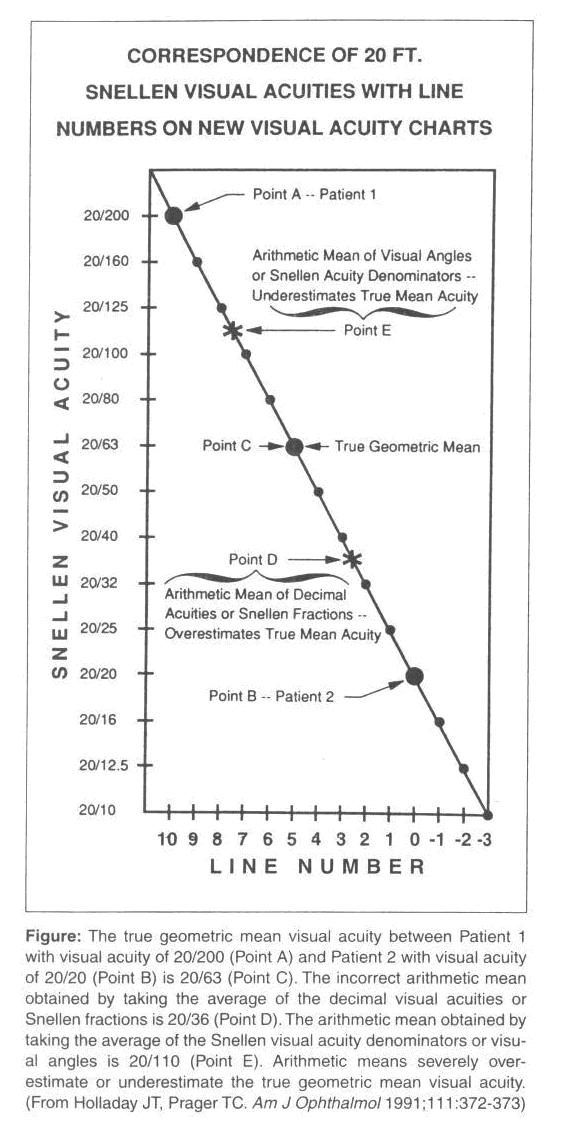 METODO APROPIADO PARA CALCULAR LA AGUDEZA VISUAL PROMEDIO JACK
…………………………ANABİLİM DALI BAŞKANLIĞINA SON 5 YILA AIT (20–20) “UÜ
 REFORMA AL REGLAMENTO DE FUNCIONAMIENTO DEL COMITÉ DE TRANSPARENCIA
RESPONSE OF BRIDGESTONE FIRESTONE TO SAVE MY FUTURE FOUNDATION
NOTA DELLA CONGREGAZIONE PER LA DOTTRINA DELLA FEDE SULLA
BUSINESS ORGANIZATIONS BULK ORDER FILE LAYOUT COMMADELIMITED PRODUCTS BULK
STEPHAN MARKS MANUSKRIPT ZUM SEMINAR MENSCHENWÜRDE UND SCHAM SALMAN
 SOCIEDAD LATINA DE COMUNICACIÓN SOCIAL [ASOCIACIÓN CIENTÍFICA NO LUCRATIVA
EXHIBIT GUIDELINES DEPT XXV COURT CLERK SHELLEY BOYLE (702)
 SOLUCIONES PRÁCTICA 3 1 TRABAJAMOS CON CINCO VARIABLES BINOMIALES
NA OSNOVU ČLANA 27STAV 2 ZAKONA O ZAŠTITI ZRAKA
CONTRATO ENTRE EMPRESA Y EL GRUPO DE INVESTIGACIÓN …………
MEMORIA DE ACTIVIDADES FAK 2013 ENERO DÍA 26
MS MESTERKÉPZÉS – SZAKINDÍTÁS II4 AZ OKTATÓK SZEMÉLYISZAKMAI ADATAI
