DO HOUSEHOLDS SMOOTH THEIR CONSUMPTION? 1 INTRODUCTION THE CASE

1. Introduction

The case study ‘Does income constrain household spending?’ considers the responsiveness of consumption to income in the long-run. Since disposable income is a relatively volatile series it is important for economists and policy-makers to understand how income affects consumption not only in the longer term when the changes have become permanent, but in the short-term, when changes may be transitory and soon reversed. Therefore, in this case study we use the concept of the income elasticity of consumption to see whether the impact of income changes on consumption depends on the length of time over which the change occurs.

2. Income elasticity of consumption

Between 1921 and 2006 the annual compound growth rate for the real values of both household consumption and disposable income was 2.3% per annum.¹ By holding consumer prices constant the year-to-year percentage change in real consumption captures the change in the volume of spending, while that in real income captures the change in the purchasing power of the consumer.

Chart 1: Quarterly growth rates

Source: National Statistics, ELMR Table 2.5

To demonstrate the relative volatility of disposable income over consumption, consider Chart 1. It shows the percentage change in real disposable income and in consumption from quarter to quarter since the first quarter of 1955. The profile of the quarterly growth in disposable income is typically more erratic than that in real consumption. Hence, while the rates of consumption and income growth are approximately equal in the long run, this is not so in the short run.

One explanation as to why the path of consumption is smoother than that of income is that the financial system enables households to borrow or save. Therefore, households can trade income across time to delay or bring forward consumption plans. This trading of income is known as inter-temporal trading.

In deciding how to respond to changes in disposable income households may form expectations as to the likely future profile of disposable income. If a change is perceived as transitory, households may change their consumption relatively little. For instance, a short downturn in income may be offset by running down savings or undertaking borrowing. The more permanent the impact on income is perceived to be the greater might be its impact on consumption.

The extent to which a change in income impacts on consumption is captured by the income elasticity of consumption. It measures the percentage change in consumption following a 1% change in disposable income.² Modelling economics relationships using a log-linear specification is popular because the coefficients can be interpreted as elasticities. The following consumption function has a log-linear specification so the coefficient on disposable income, Y, is the income elasticity of consumption.³ The subscript t represents a moment in time.

(1)

The log-linear function can be derived from the power function

(2)

The income elasticity of consumption, , is the fixed power by which the variable base income, Y, is raised.  is a scalar simply moving the values of Y^ up or down.

Chart 2: Log-linear consumption function

Source: As Chart 1

Chart 2 is a scatter plot of combinations of consumption and disposable income at constant prices in common logs from 1955Q1. The common logarithm is the logarithm with base 10, written as log. The log-linear consumption relationship is estimated by a line of best fit. This is the straight line that best represents our data points.⁴ The vertical distance between the line and the observations measures the error in the estimated consumption relationship.

The equation of the line of best fit has an intercept of 0.227 and a slope coefficient of 0.97⁵, such that

(3)

From this, we infer that a 1% increase in real disposable income results in real consumption increasing by 0.96%.

The relationship specified in equation (1) is a levels relationship because it models the determination of the level of consumption. But, because the level of consumption can be compared between two periods as the level of income changes, it can be transformed into a growth relationship.

Imagine that two snapshots of consumption are taken. One is taken at time t and the other i periods earlier, at time t-i. The level of consumption at t and t-i is dependent on income at the corresponding time, such that

(4)

(5)

A change in income causes a change in consumption. The change in consumption is found by subtracting (5) from (4)

(6)

This is equivalent to

(7)

After factorising we find that the difference between consumption in the two periods is

(8)

The quotient rule of logarithms is that a subtraction ‘outside’ of the log can be turned into a division ‘inside’ the log. The subtraction of our two log consumption values can be written as

(9)

The quotient ‘inside’ the log on the LHS of (9) is the relative value of consumption in period t to that in period t-i.

The subtraction of our two log income values can be written as

(10)

The quotient ‘inside’ the log is the relative value income in period t to that in period t-i.

Each quotient is a scale factor. A scale factor is a measure of change or growth. A scale factor of greater than 1 means that the final value exceeds the original value whilst a value of less than 1 means that the final value is smaller than the original value. So, for instance, a scale factor of 2 for consumption means that that the final value of consumption is twice the original value. In other words, there has been a two-fold increase.

Equation (8) models the scale factor for consumption and so its rate of change. However, in representing change it is convention to use the upper case Greek character , pronounced delta. Consequently, the change in the log values of consumption and in income in period t from period t-i can be written as

(11)

(12)

Therefore equation (8) can be written more succinctly as

(13)

Equation (13) is a growth rate model derived from a levels specification. It contains no constant and the slope coefficient is the income elasticity of consumption, . Therefore, theoretically at least, if we estimate  using either the levels model captured by (1) or the growth rate model (13) we should get the same value.

Rearranging (13) we can write the income elasticity of consumption as

(14)

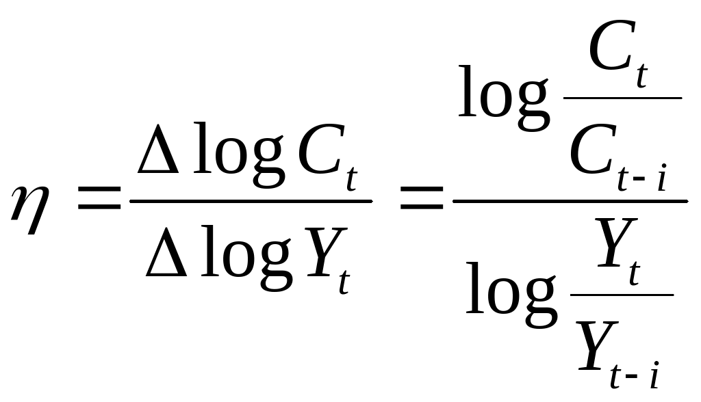
Equation (14) shows the income elasticity, , to be invariant to the number of periods, i, over which the change in consumption and income is measured. It is this assumption that we now consider.

3. Empirical analysis

In modelling the growth in consumption, as in equation (13), the number of periods over which to measure the change has to be chosen. The frequency of the available data goes a long way to determining this. If we have annual data then the shortest period of change we can analyse is between one year and the next.

Quarterly data gives us the flexibility of modelling quarterly and annual growth in consumption.⁶ The former enables consideration of very short-run changes in income, while the latter allows consideration of income effects on consumption which, whilst still short-term, are less transitory.

Chart 3: Quarterly growth

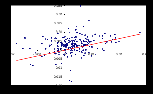
Source: As Chart 1

Chart 3 is a scatter plot of combinations of quarterly changes in the common log values of consumption and disposable income from 1955Q1. A line of best fit is used to estimate equation (13) and so be our simple model of quarterly consumption growth. The line best fitting the data is

(15)

The income elasticity is estimated to be 0.33. This is considerably less than the value of 0.96 inferred for the elasticity when the levels relationship (1) is estimated.

Chart 4 is another scatter plot, but this time for annual changes in the common log values of consumption and income from 1955Q1. Calculating annual growth rates with quarterly data involves comparing the same quarter of two consecutive years.

Chart 4: Annual growth

Source: As Chart 1

The equation of the line of best fit and our model of annual consumption growth is

(16)

The income elasticity this time is estimated to be 0.78. Therefore, by increasing the period of change from 1 quarter to 4 quarters, the impact of income on consumption, as measured by the income elasticity of consumption, increases.

By comparing the income elasticity estimated from our growth rate models and our levels model, we infer that total consumption is more sensitive to income in the long run. Further analysis could consider whether this holds for different types of household expenditure, such as consumer durables, semi durables, non-durables and services. It could also compare the responsiveness to income across these (or more disaggregated) categories of household spending. This would help to further our understanding of the determination of household spending.

Tasks

1. Evaluate the following logs

1. log₄16

2. log₁₆4

3. log₁₀1000

4. log₂¼

2. Evaluate the following

1. log₁₀10,000 – log₁₀100

2. log₁₀(10,000/100)

What rule of logs have you demonstrated in answering (a) and (b)?

3. An economist decides to construct a model of the level of household consumption as well a model of its growth from period-to-period. Why might they be doing this? And do you think this should be done for other economic relationships?

4. Would you expect the income elasticity of consumption to be smaller in the short-run than in the long run for all types of household spending?

1 The compound growth rate formula can be written as where A and V are respectively the first and last numbers in a series and where n is the number of periods.

2 It can be written as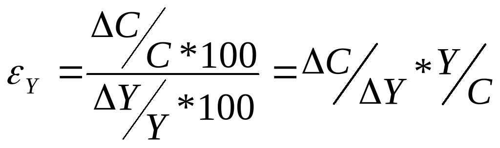 whereC and Y are the change in consumption and income respectively.

3 The logarithm of a number y with respect to a base b is the exponent to which we have to raise b to obtain y. Therefore, log_by = x means b^x = y.

4 This can be done in Excel by using the Add Trendline option in the Chart menu. By then ticking the appropriate box in the Options menu the equation of the line is displayed.

5 The income elasticity value of 0.96 compares with the estimated value of 0.97 in the case study ‘Does income constrain household spending?’ In that study the data was per capita (per person), of an annual rather than quarterly frequency and available from 1921, when the current borders of the UK were established.

6 The frequency of data should not be confused with the type of growth rate. For instance, an annual growth rate can be measured using a monthly data set simply by comparing the same month in two consecutive years.

4