SPACE BASED AUTOMATED MODULE METHODS OF TRAJECTORY AND DOCKING

DUALUSE LIST CATEGORY 9 – AEROSPACE AND
JOB TITLE GROWING GREEN SPACES COORDINATOR HOURS 14
SOMMAIRE 1 L’ENVIRONNEMENT DE L’ESPACE DE VIE

---

THE SPACE AFTER THIS TEXT IS NEEDED TO
!DOCTYPE HTMLHTML LANGENHEAD META CHARSETUTF8 BASE HREF TITLEDSPACE REPOSITORY
&ADKEYWORD &ADTYPE &ADCOUNT &ADNAME &ADSERVER &ADSIZE &ADSLOT &ADSLOTS &ADSPACE

---

A principal scheme of calculations of control algorithm with 'model' is described in the paper

Space Based Automated Module. Methods of Trajectory and Docking Control.

Authors: M. Pivovarov, A. Zakcharov, G. Veselova, E. Djujeva, L. Blinova, I. Sidorov, V. Frolov.

Space Research Institute of Russian Academy of Science

Preface

Principal schemes of flight control methods elaborated by specialists from the Space Research Institute are described in a given address. As an object of control an automatic Space based module, capable to execute a set of dynamic operations in the Orbital Station environs is overviewed.

The main technological tasks the module should execute are as following:

1. Flying up to the object, which is moving near the orbital station, docking with it, towage and assembling an object at a given place at the orbital station;

2. Carrying out different objects from the station and providing their trajectory of flight and angular orientation as need be;

3. Re-docking station modules or fragments of construction from one place to another;

4. Flying around the station and hanging in a given point in order to carry out the visual inspection of the station’s external surface;

5. Performing the maintenance at the external surface of the station.

It is shown that the module's control system and corresponding motions control algorithms are able to ensure the exact realization of mentioned above tasks.

1Automated Module Main Sub-systems

The free-flying universal automated module (AM) has its own control system capable to ensure the spatial controlled motion of AM center of masses and spatial angular turns about center of masses. The system can operates in two working modes - completely autonomous mode, when the system realize a preliminary determined set of operations using the corresponding algorithms of autonomous control; and second one is an operating in a dialog mode by means of commands received from operator at the Station.

To realize the mentioned above technological activity the AM control system should consist of the following main blocks (the control system doesn't include the manipulator itself):

1. Autonomous navigation system (ANS). ANS consists of three accelerometers; each measures the current AM acceleration along the corresponding translational coordinate constrains with AM. We assume an accuracy (error) of acceleration measurements g ~ 2.10^-5 m/s². ANS also include three angular velocity detectors for measuring the current angular velocity about each axis constrains with AM. We assume an accuracy (error) of angular velocity measurements  = 20 arc.min/hour. ANS has a specialized on-board computer for calculating on the base of special program the current values of absolute translational coordinates, velocities, angular coordinates and velocities. This information incomes into the AM main on-board computer.

2. Position-sensitive optical system working in complex with marked beacons (point-like sources) fixed near the setting place of an object to dock with. Towards each beacon the detector measures two spatial angles ,  in two planes between the optical axis and line directed towards the beacon. The geometrical scheme of angle measurements will be represented below. To provide the satisfied accuracy of angle measures to use the detector with light-sensitive matrix, having 512 x 512 elements, is enough. From our point of view to use the focus transform device to change the field of view angle is desirable. Market beacons should be located not only near the setting place but also in some predefined points at the Station and other objects the AM operates with. The detector (as one of the version) may be supplied with mini-driver for the optical system angular turns.

3. Low-thrust pulsing jet engines. The engine is a rather small electric-magnetic valve, capable to realize short pulses. In calculations we accepted that the minimal duration of pulse the engine is capable to produce is 0.01 s. The working body of engine is a two components fuel. To realize the required AM spatial control along translational and rotational coordinates we examined few versions of engines number and their relative location at the AM. The possible number of engines may be 12, 16, 20, and 24. But the detail solution of this task and searching for the optimal scheme should be done during the platform elaboration at the next stage of the work.

4. On-board computer processes the original data received from ANS and optical system, executes the corresponding algorithms of control and sends commands to actuate the particular pulse engines.

5. Radio system for linking AM with operator at the Station and exchanging the information important for the control. We suppose that radio will be used when the AM operating in dialog mode.

6. We also include here the automatic system for fixing the platform at the setting place. The device, we propose as a docking unit, consists of two magnetic plates having the cross-polarized magnetic field. Depending on plates relative angular position the force of attraction may be varied from zero to the nominal value. Here with the magnetic field acts practically at a distance from the plate surface of about 2 mm. To ensure the AM fixing the docking place of an object should be supplied with the small iron plate. The nominal attraction force is 6 kg/sm² and the plate with squire of about 50 sm² installed at the docking place is enough to provide the attracting force about 300 kg. By the rotating one of the magnetic plate at an angle ~ 70⁰ an attraction will be reduced up to zero and the AM may be separated with an object.

From our point of view the AM operating capabilities is convenient to represent as a set of operating phases the AM should realize in an Orbital Station environ. These phases are combined into a single technological cycle, which is represented at fig 1-1

Initial conditions are: at a distance ~ 5000m from the Station flies an object ( let it be a kind of technological satellite). It is supplies with marked beacons on the external surface. The AM task is to deliver this object to the docking place at the Station.

The cycle of operations the AM should perform consists of the following phases.

Phase 1. The unloaded AM is separated with the Station by means of short pulse and is installed at the nearby orbit (it may be the circular orbit) with relative altitude ~ 50m. Using the preliminary information on an object relative location and relative velocity AM orientates towards it. Observing the market beacons by means of optical detector AM specifies its position relative to the object.

Phase 2. By means of selected beforehand control method AM flies to the object environ.

Phase 3. AM executes the approach and docking with a given object. Let us call the new system (AM + load) as the loaded AM.

Phase 4. Loaded AM executes the required angular turns and flies back to the Station environ.

Phase 5. The loaded AM is set at the appropriate trajectory of flight around the Station to ensure the satisfied dynamical conditions at the initial stage of approach process. Then on the loaded AM executes approach and docking at a given setting place at the Station. With this phase the cycle of operations is finished.

It is easy to see that all others mentioned above operations (except AM operating in "inspector" mode) may be represented as combinations of tasks performed within this cycle.

The exact and reliable accomplishment of mentioned above maneuvers is based on application of corresponding algorithms of AM motion control. The main contents of these methods are described below.

2Long Range Flight Control

2.1Position/Orientation Determination

To determine the AM relative spatial coordinates and velocity vector we propose to use one position-sensitive detector and one marked beacon located at an object to dock with.

This version will be applied when the distance to the beacon is rather large (~10000m.) and the detector cannot resolve reliably two beacons because of the limited angular resolution. In this case the scheme of consecutive measurements in a given time intervals t_i was elaborated and rather good results were received.

Overview the calculation schemes, considering that the platform orbit coincides with the orbit of an object to dock with (orbital station or some kinds of satellites). Let us call this object - a target object. The duration of flight is around 5000 s. and typical relative velocity is less than 10m/s.Under these conditions the position-sensitive detector continuously observes the marked beacon placed at target object and measures value of an angle (t) between the optical axis and line towards the beacon (optical axis and beacon lie in the orbit plane). Here with we assume that during the autonomous flight a rather high errors is accumulated when calculating the platform relative position and velocity.

Calculations are done in coordinates system constrained with the detector.

(Z₀ - along optical axis, X₀ and Y₀ are in the plane of detector's light-sensitive matrix). The detector location relative to the platform's center of masses is known a'prior.

To simplify calculations we consider that the platform is orientated towards an object so that the beacon lies in coordinates plane (Z₀,X₀) of the detector, conformably the plane (Z₀Y₀) is perpendicular to the orbit's plane. This version of the platform relative location is the most simple and convenient to calculation. The corresponding scheme is depicted at fig.2.1-1

The procedure of position and velocity determination in this version is as following.

At a given initial moment t₁ (the platform is far from an object) the onboard computer has the preliminary information on values dL_E and dr_E received for example from ANS, where:

dL_E - an estimated distance to the object along the detector's optical axis (Z₀);

dr_E - an estimated distance along X₀-axis

Let us consider that at the initial moment t₁ the accumulated relative errors have the following values:

- along Z₀-axis Z and ;

• along X₀-axis X and

The aim of calculations is to estimate errors Z, , X and and thus to get the accurate data on platform current spatial position and velocity vector.

At a given time t₁ the true values dL and dr are as following:

(2.1.1)

In a time interval t₁ = t₂-t₁: (t₁ ~ 100 - 150 s.) at a moment t₂ the second set of

m
easurements is take place.

(2.1.2)

where : L₁ - an estimated distance along Z₀-axis within the interval t₁ ;

R₁ - an estimated distance along X₀-axis within the same time interval.

Values L_1, R₁ are received from the direct integration of exact motion equations. The interval between measurements is rather short and we assume that within this time interval t₁ no errors are accumulated.

In time intervals t₂ =2t₁ and t₃ =3t₁ we have the same relations for dL and dr at points t₃ and t₄ respectively:

(2.1.3)

(2.1.4)

Detecting the angle _n (n = 1,2,3,4) at the corresponding points t₁, t₂, t₃, t₄ we receive in accordance with the geometrical relations the following system of linear equations:

(2.1.5)

Using relations (2.1.1 - 2.1.4) we may find the solution of the system (2.1.5) and to determine values Z, , X and . Substituting these values in equation (2.1.4) we may find the first approximations of relative co-ordinates and velocities dL, dL', dr, dr' for the current time t₄. One should note that in the scheme we assume that no errors are accumulated within the time interval t₂ and t₃ as well.

According to accepted scheme of detector spatial position, its Y₀ -axis is perpendicular to the orbit plane. Detecting the corresponding angles (t_n) in the plane (Z₀Y₀) we may use relations similar to 2.1.1 - 2.1.5 to determine errors Y and along this direction. We should make at least two sets of measurements, for instance at point t₁ and t₂. In this case the relations for the true values Y(t_n) will be as following:

(2.1.6)

(2.1.7)

Values Y_E and Y₁ are the estimates of translational co-ordinates along Y₀-axis received from integration of motion equations as well.

Two additional equations to calculate Y and are as following:

(2.1.8)

These equations should be added to the system (2.1.5). The final system consisting of (2.1.5) and (2.1.8) allows to determine the full amount of errors and to estimate precisely the current platform position.

We may continue the described above sequence of calculations for another time intervals until the platform is in the environs of an object to dock with.

The calculations done according this scheme give the following preliminary results:

When the distance to the docking place is ~ 500 m. we may decrease the current time intervals t_n up to 20 - 40s. and therefore to upgrade the accuracy of received results. At the initial step of approximation (for time interval t₁ - t₄) the accuracy of relative translational co-ordinates (L,R) determination is around 5m, the relative velocity accuracy is 3 sm/s. At the terminal point (the relative distance  300 - 500m) the final accuracy of co-ordinates determination ~ 20 sm., relative velocity  0.5 sm/s.

In calculations we assume the acceleration measuring accuracy ~ 2.10^-5 m/s².

On the base of given calculations the preliminary technical requirements to the detector are formulated:

- system must be capable to record the angular position of beacon within the distance range 1 and 10000 m.;

- field of view angles range 5⁰ - 15⁰ ;

- the accuracy of beacon angular position measurement 1' - 3 ^';

- the rate of data interrogation from the sensor ~ 10 to 20 Hz;

- it is desirable to use the focus transform device to change the field of view angle.

2.2Dynamic Equations Analysis and AM Transition to the Environs of an Object to Dock with

Within the limits of this paragraph we shall overview the following procedure of the platform flight control.

The initial conditions are as following:

It is considered that an orbit planes of platform and an object of docking are coincided. The initial relative distance  10000m., the typical relative velocity  10 m/s. The based trajectory of an object flight is a circular orbit with an altitude 450 km. and period 5610s. (it is approximately corresponds to the orbit of an International Space Station).

The aim of this phase of flight control is to ensure the platform flight from initial point having arbitrary relative co-ordinates and velocity to the terminal point (null point) located near the docking place of target object.

The optimal method of control at this phase is a three-pulses maneuver executing during the time interval equal to the period T_p of target object's revolution round the Earth (in our case T_p=5610s.). Here with the third pulse as usually is needed to decelerate completely the satellite at the moment the docking is taking place. The distinction of proposed below method of control is that to construct the process ensuring in the terminal point a smooth and without hanging passes to the next phase of flight in the docking place environ. That is why during the flight only first two pulses are executed and the final decelerated pulse is partly prolonged to the next flight phase. Another difference is constrained with selecting the certain co-ordinate system and dynamic parameters allowing to get rather simple analytical relations of control pulses. This in turn allows to simplify the selection of terminal dynamical conditions (this conditions will be the initial parameters for the second phase) and to pass accurately to the next phase of control.

Overview the initial system of platform motion equations

(2.2.1)

Where: v - orbital velocity, r - altitude of flight,  - pitch angle, L - distance along the Earth surface, z - deviation towards the perpendicular to the orbit's plane, P_x - engine's power projection at the velocity vector, P_y - engine's power projection at the Earth radius-vector, P_z engine's power projection at the perpendicular to the orbit's plane, m - platform's mass, R - Earth radius, g₀ - earth gravity at the surface.

g₀ = 9.81m/s²

The system of equations in decrements is received when substituting the variables in system 2.2.1

Where: variables v₀, r₀, L₀, =0 describe the motion of target object along the circular orbit.

The corresponding system of equations has the following form:

(2.2.2)

Where: c₁ =2/v₀ , c₂ = ²/v₀, =2/T_p

The determinant of the system is as following:

D() = - ²( ² + c₁g₁ –v₀c₂)

The determinant nonzero roots are:

 =   ,  =1.12*10^-3 1/s

The value T_p = 2 / = 5610s.

Overview the first four equations of system (2.2.2 ) describing the platform motion in the orbit's plane. The last equation describes the motion in the perpendicular direction. It doesn't connected with other equations and will be overviewed later.

It is convenient to make one more substitution of variables in system (2.2.2 ) using the following relations.

x = ( c₁dv +c₂dr )/ , u =dv + dr (2.2.3)

The new system of dynamical equations is:

(2.2.4)

The reverse transformation of variables gives the following relations:

dr = - x/c₂ +c₁/c₂ u , dv= -u +v₀ x

Analyzing system (2.2.4) one should note that the first equation is separated from others and in case P_x = P_y =0 the value u=const along the trajectory of relative motion. Second and third equations describe the rotating mode of the platform relative motion with period T_p and the last equation is an integral of motion along dL co-ordinate. These equations for example allow to make the following simple conclusions. Providing u =0 and x = const, all over the period T_p we should have the relative motion along a stable in time elliptic orbit with parameters depended on value x. Here with the value u 0 determines the ellipse shifting in time along relative co-ordinates (dL,dr). Besides, this system shows that the power pulse P_x is a two times effectively than P_{y .} Therefore from the point of view of fuel consumption it is better to apply the control pulses when d =0 and to repeat them each half a period (if it is needed).

In general from our point of view the proposed equations (2.2.4) are very convenient for analyzing the current dynamic process and their application significantly simplify the control task solution.

Overview in consequent orders the solution of mentioned above control task. In co-ordinate system constrains with the target object at the initial moment t₀ relative co-ordinates dL₀ ,dr₀ as well as initial velocity vector dv=dL' + dr are calculated (using 2.1.5 and 2.2.2). The task is to transit the platform during the period T_p from the initial location to the terminal point, constrains for example with the target object ( dL=0, dr=0, dv=0). In variables dL, u , x it is equivalent to transition the platform to a point with co-ordinates dL=0, u=0,x=0.

To determine the velocity pulses values correcting the current trajectory of flight we shall overview three versions of initial conditions.

1. At the initial moment t₀ (let us consider d(t₀)=0) values dL0, u=0, x=0. It means that the platform and the target object are at the same orbit at a distance dL and the relative velocity dv=0. To shift the platform at a distance -dL along the orbit we may get the corrected pulses directly from the last equation of system 2.2.4

Jm₁₁(t₀) =dL/3T_p , Jm₁₃(t₀ + T_p) = -dL/3T_p (2.2.5)

Under the construction of pulses variables (u,x) would have the following values:

At the initial moment u(t₀)= Jm₁₁(t₀) , x(t₀)= Jm₁₁(t₀) c₁/;

At the terminal point u(t₀ + T_p)=0, x(t₀ + T_p)=0, dL=0. (the required conditions are achieved).

2. At the initial moment dL=0, u0, x=0

On the base of equations (2.1.3.4) we shall derive the following values of velocity pulses:

(2.2.6)

These sequences of pulses were received with the help of simple conclusions. After the first pulse variables would have the following values: u₁ = u/4 (remaining of u), x₁ = -c₁3u/4.

After half a period T_p/2 the velocity u₁ and the corresponding distance dL₁ should be compensated during the remained time T_p/2. By the second pulse (-u/2) the remained values will be: u₂ = -u/4. Variable x₁ after half a period will change the sign (x₁ = c₁3u/4) and executing the second pulse the value should be:

x₂= (3u/4-u/2)c₁/=c₁u/4.

At the terminal point (t₀ +T_p) the distance dL₁ will be compensated (the whole dL=0). By the third pulse (u/4), as it is clear from the previous relations, variables (u,x) will be set to zero (u=0,x=0). Again the required conditions are realized.

3. At the initial moment dL=0 , u = 0, x0.

This version may be excluded by executing an additional first pulse.

From the relation 2.2.3 it is resulting that to set x to zero the current velocity should be:

dv = -drc₂/c_{1 .} Here with value u= u₀ =dr/2

To achieve it one should add at the moment t₀ the pulse value

Jm₀(t₀)=-(dv+drc₂/c₁), (2.2.7)

and therefore to provide at the initial stage of control the value x=0. By this additional pulse we reduce the situation to the previous version with corresponding value u₀.

Finally having the arbitrary initial values dL ,u, x, we may fined the values of control pulses by summing the corresponding pulses in relations 2.2.5, 2.2.6 and 2.2.7.

(2.2.8)

Using the same system 2.2.4 and applying the same reasoning we may modify the pulses to ensure the platform transition to the terminal point with relative co-ordinates r, L. It is easy to ague that in this case in relations 2.2.3 instead of dr we should take dr_f = dr-r and in equations (2.2.8) instead of dL should be dL_f = dL - L - 6r. Besides, to ensure at the terminal point the value dv=0, the additional terminal pulse p = r should be executed.

Under these conditions the general structure of pulses is as following:

(2.2.9)

Parameter  may have the following value:

 =1 - relative velocity dv = 0 at the terminal point;

 = - 1 - the platform will be set at an elliptic orbit around the target object;

 = 0.5 - the platform will be set at a nearby circular orbit with radius (R+r₀)+r

In the direction (z) perpendicular to the orbit plane we have the following dynamic equation:

At the initial moment t₀ the relative co-ordinate and velocity along z are:

In this case to coincide orbits two pulses should be executed at the moment t₀ and t₀+T_p/4 respectively. The corresponding pulses have the following values:

(2.2.10)

The whole amount of pulses determined in 2.2.9 and 2.2.10 ensure the platform controlled flight from the arbitrary point to an environ of an object to dock with. Here with the proposed system of equations 2.2.4 provides a rather simple procedure of control pulses determination and allows to go away of complicated calculations. Manipulation with variables (u, x) considerably simplify the analyze of platform dynamic, ensuring therefore a smooth passes to the required initial conditions of the next stage of control in the close environ of target object.

3Approach and Docking Phase Control

3.1Position/Orientation Calculating Scheme

To construct the platform control algorithm when flying in the station environ to have the information on platform current spatial coordinates and velocities relative to the station is needed. As it was mentioned in Chapter 1 (task 6) to calculate the AM current position and orientation two types of measuring instruments are applied.

1. autonomous navigation system consisting at least of three angular velocity detectors, tree accelerometers and a specialized computer;

2. position-sensitive optical system working in complex with marked beacons (point like sources) setting near the docking place.

Within the frame of given researches tow versions of calculations schemes enabling to determine the AM relative spatial position and angular orientation were examined.

Integrating system of dynamic equations and using data from ANS the on-board computer has an information on AM current spatial coordinates (position and orientation) and velocities relative to the Station. Using the calculation procedure mentioned in paragraph 2 the algorithm of control at each current time interval has an information on the platform coordinates and velocities relative to the target object and its docking place respectively. Here with the rotational coordinates are determined with high accuracy but the translational values have an insufficient accuracy to ensure an approach control.

The initial conditions of AM autonomous flight are as following:

• AM autonomous flight time is rather shot (around an hour) and the original data coming out of angular velocity detector are rather accurate;

• The initial distance between detector and marked beacons < 200 m.;

• Beacons are in the detector's field of view;

• The platform flies towards the docking place.

In this case to determine the AM location we may use one optical detector and two marked beacons, fixed near the setting place of the object AM have to dock with.

At fig.3.1-1 the schematic of AM spatial location relative to the docking place is depicted.

fig.3.1-1

Co-ordinates system (X₁Y₁Z₁) constrained with the platform's centre of mass. Co-ordinates of detector (D) in the co-ordinates system are , i.e. (X₀,Y₀,Z₀) is the shifting of at value (a) along X₁ axis. The co-ordinates system is constrained with the center of mass of an already docked AM. In co-ordinates system (XYZ) co-ordinates of marked beacons 1, 2 are (a,b,0) and (a,-b,0) respectively.

The detector (D) provides the onboard computer with information on two pairs of angles (₁, ₁) and (₂, ₂) between the detector's optical axis (O_Z) and corresponding beacons (1,2) as it is shown at fig.1.

It is convenient to calculate the current AM translational coordinates in system (XYZ), constrained with the object's docking place.

Solving the geometrical task, we receive in the coordinates system coordinates of the platform's center of mass, its altitude over the support place and the angular position _Z about the vertical axis.

(3.1.1)

(3.1.2)

(3.1.3)

(3.1.4)

where:

.

.

_X and _Y - platform orientation about X and Y axes respectively.

One should mark that within a given scheme of relative location at the initial phase of docking control values _X and _Y are rather small and are reduced to zero near the terminal point. That is why during the whole process the calculated relative coordinates have a satisfied accuracy.

Finally along with angular coordinates, received from the angular velocity detector, we have in real time scale the full amount of data on AM current spatial location.

3.2Algorithm with ‘Model’ and Terminal Task Methods Application

From our point of view the most critical element of flight is the approach and docking phase. In this respect to ensure a high stability and accuracy of dynamic process control an algorithm with "model" and original scheme of terminal task solution was elaborated. Even this task attracts the main attention in our researches.

The proposed method of control executes in consecutive order the following operations. On the base of data, incoming from an autonomous navigation system or optical system (when observing marked beacons), it determines the current coordinates of the platform relative to the station, its spatial angular position, as well as components of the velocity’s vector and disturbing external forces.

Have used a selected beforehand law of the platform moving and solving a corresponding terminal task, we receive the current values of required engine’s power. Having analyzed the calculated results, the control system actuates particular engines of the platform and corrects the trajectory of flight as need be.

The algorithm permanently repeats the above-described procedures with periodicity ~ 0.1-0.2 sec. until the process is completed.

To show the principal scheme of the control algorithm, let us overview a concrete process of approaching and docking of the platform at a given place on the surface of the station.

First of all, it is convenient to calculate current translational coordinates and velocities of the platform in the coordinates system (XYZ), constrains with the docking place of the target object. Coordinates X, Y are in the plane of docking surface and plane (X,Z) coincides with the orbit plane.

Let us overview the processes of control in the plane of the station orbit.

The initial conditions of the task may be as following:

• relative distance along Z-axis is around 150m;

• relative velocity of approach is less than 1.5 m/s;

• relative velocity of docking is less than 0.15 m/s;

• detector's plane is orientated towards the marked beacons.

Within the process the following random disturbances may be: deviation of pulse power from the nominal value, shifting of the platform’s center of mass and change of inertia moment (due to the fuel expenditure), low-frequency flexible oscillations of setting place.

In proposed method the platform motion near the setting place may be described by the simplified system of dynamic equations (“model”), where the external forces and disturbances are low then the power of a low-thrust engine. We should mark that depending on particular platform initial location, along Z-axis might be either relative distance along the orbit (dL) or relative altitude (dr). Along X-axis would be variables (dr) or (dL) respectively.

Examine the principal scheme of the control algorithm. Let us assume, for example, that the docking place is at the "top" side of the station and at the beginning of approach phase the platform moves towards the docking unit along the relative altitude dr. Initial versions of approach phase is depicted at fig 3.2-1 along with the corresponding controlled approach trajectories

At the initial moment the marked beacons, fixed near the setting place, come into the detector's field of view. From then on, the algorithm solves in consecutive order the following tasks.

1) The position-sensitive sensor feed the on-board computer with information about the angles between the marked beacons (it is enough two beacons) and

detector's optical axis Oz . Solving the geometric task (described in § 3.1), we receive in the coordinate system (constrained with the center of mass of

the already installed platform) coordinates of the platform's center of mass, distance L along Z-axis and the angular position _Z about Z-axis.

2
) Calculations of components of the velocity’s vector and estimation of disturbing forces values are done with the help of algorithm with "model" procedure.

In co-ordinates system (X,Z) it is convenient to use the following dynamic equations of the platform motion ("model"), where external forces are absent.

(3.2.1)

where: , Y_m, Z_m - coordinates of the platform relative to the setting place;

, P_Y, P_z - power of pulse engines;

- platform’s mass.

Choose the interval of analysis , where:

- time interval of feeding the on-board computer with data from the detector

( = 0.1 - 0.2s);

- number of points at the interval (n = 50- 100).

At the first interval of analysis P_x=0

Let us overview the control process along X-axis.

By a point-by-point integration of equations 3.2.1, at each step of integration we have the estimated values of coordinate X_m(n) and velocity V_Xm(n). Then, at the interval of analysis at each step differences are calculated:

(3.2.2)

The received values are approximated with parabola with the help of less squares method and at the end of the interval T increments of coordinate X , velocity V_x (derivative of parabola at the end interval T) and disturbing external forces F_Xq (second derivative of parabola) are calculated:

(3.2.3)

where:

- weight coefficients (coefficients of approximation) having the following construction:

(3.2.4)

where: N=T/2t and should be an integer number, n = 1, 2, …2N

a = 2 for even numbers, a = 4 for odd numbers and a = 1 at the end of interval of analysis.

We take the parabola on the base of assumption that the relative evolutions of the platform are rather slow. So at each interval T we may consider all external forces (including random disturbances) not included at equation (1) are constant. (In some cases, when the relative velocities are rather high, we may take cubic parabola). From the other hand, as it was mentioned in § 2.2, variables dr, dL (in our case Z_m , X_m) have the sinusoidal law of motion with the period T_p = 5610s. In our case the time of analysis (T  10s) consists a small pies of period T_p and therefore curves defined in 3.2.2 may be approximated with parabola with high accuracy.

Finally, the smoothed values of coordinates and velocities for the right margin of the interval T are as following;

; (3.2.5)

(It is obvious that for coordinates Z, the scheme of calculations according to relations 3.2.2 - 3.2.5 is the same).

We ought to mark, that the proposed procedure with "model" allows to calculate values (3.2.5) and force F_q with high degree of accuracy. It becomes possible because at the interval T we manage a relatively rich statistics, though we use the simple form of dynamic equations (3.2.1) and calculated on the base of data received from the detector coordinates have a rather poor accuracy.

3) Calculated values (3.2.5) and force F_q allow to solve the terminal task and to form commands for actuating particular engines ( ) as need be.

Examine the scheme of the terminal task solution along the -axis.

First of all we should estimate the duration T_k of controlled process.

At the initial moment t₀ we have the corresponding boundary conditions:

for = 0 (right margin of the interval )

coordinate (3.2.6)

velocity

To estimate the value T_k at first approximation we simply integrate the system 3.2.1 using the initial value 3.2.6. We ought to mark here that the initial velocity along Z-axis V_z  0, that is the platform moves towards the docking place and as it will be described below the control along Z-axis is reduced to the task of platform deceleration up to the appropriate value.

From the first equation 3.2.1 we shall have the following relation:

(3.2.7)

We propose to solve the terminal task in the following way. Let us choose the trajectory of flight along X-axis which satisfies the boundary conditions at the terminal point. These conditions are:

for (the terminal point)

The corresponding law of motion may have the following form;

(3.2.8)

where: C₀ and C₁ are an unknown constants.

(The problem of selecting the appropriate law of motion will be described in our next address.)

Using an equation (3.2.8) and its first derivative while t=0 along with conditions (3.2.6) we obtain the system of algebraic equations relative to and :

(3.2.9)

The second derivative of relation 3.2.8 is:

(3.2.10)

Substituting C₀ and C₁ from 3.2.9 into this relation and replacing T_k with (T_k-t) we shall receive from 3.2.7 the final relation for the required value of power:

(3.2.11)

In this relation X_s(t) and V_Xs(t) are the current coordinate and velocity along X-axis. The value (T_k - t) is the time remained to the end of the process. This parameter is permanently recalculated during the control process. Besides, to avoid the dividing by zero in this relation, when the platform is near the terminal point, we simply put over the following arbitrary condition: if (T_k - t)  0.05s then (T_k - t) = 0.05s. (but the calculations show that in fact there are no needs of this condition).

To make sure the marked beacons are in the detector field of view during the control process one more additional limit is usefully to set up. The detector field of view is limited by the angle _MAX. If in the orbit's plane the current angular location _i of one of the beacon is near _MAX (for instance _i  0.9_MAX ) then in relation 3.2.11 instead of (T_k - t) should be the value:

where: Z_i - the current altitude over the setting place;

P - the nominal engines power along X-axis;

 - an arbitrary parameter within the range (0.1  1)t.

Under this condition the calculated power P_X is depended on _MAX and the control system will always ensure beacons location in the detector field of view.

On the base of calculated value (3.2.11) the control system can ensure a required trajectory of flight at each time interval by means of pulse engines. But at the platform, we have the pulse jet engines with not adjusting engine's power P, so to execute the correct pulse value the following rule is stated: during each interval we ought to produce the power pulse Pt, where

t = .

But the value t is limited by the minimal pulse duration the engine is capable to realize. For the pulse engines we propose to install at the platform t_min = 0.01s. So, if t  t_min the engine is not switched. (The computer simulation of control process shows that normally the value t  0.5 t )

The engine switching is realized by the command from the computer.

Then on the algorithm repeats the whole above-described procedures through relations 3.1.1 - 3.2.11 during the second time intervals (shifting the current interval of analysis at step ) and so on until the process is completed.

One should note that in correlation (3.2.11) the item in fact plays a role of dynamic stabilizer of the process, damping different disturbances occurring during the flight.

Along Y coordinate the relation for power P_Y is similar to relation 3.2.11

Concerning the control along Z-axis we may repeat absolutely the same procedure through 3.2.1 - 3.2.10 replacing with and to get the same relation for P_z.(but without first term).

(3.2.12)

The reason of excluding the term connected with the relative coordinate is the following. According to the accepted dynamical scheme Z-axis is perpendicular to the docking place and the platform moves practically along this direction. That is why the process of control is reduced to the deceleration of the platform, so the term has no means and should be excluded in relation 3.2.12. From the other hand during the contact with the setting place the platform should have a negligible velocity to provide the docking. To ensure this regime we should receive the following rule: if V_Z (t) V_min then V_Z=0 (V_min might be, for example, 0.1m/s.).

The corresponding trajectories of controlled flight for different versions of initial conditions are represented at fig 3.2-1.

From our point of view the proposed algorithm of control is rather universal and may be applied in different versions of platform motion in the object environ, including the platform angular attitude control. In this case to control for example the angular position and angular velocity about Z-axis we may use the equation:

(3.2.13)

where: - angular acceleration about Z-axis;

M_Z - momentum about Z-axis;

J_Z - inertia abour the axis.

Applying the described above procedure of calculations with the terminal conditions ( ) we shall receive the relation for the value M_Z

(3.2.14)

M_Fz - accidental angular disturbances (also calculated within the algorithm with "model".

To realize the platform angular stabilization within the limited angle and limited angular velocity when executing an approaching phase we should choose the appropriate value (T_k - t). Thus to make the relation (3.2.14) sensitive towards the angle     _max the following condition should be fulfilled:

(T_k -t)  T_min = (J_Z12_max / pM_max ) (3.2.15)

where: M_max - the available (nominal) momentum value;

p - parameter which in fact is an equivalent of minimal pulse duration the engine is capable to realize. In our case p =  t _min / t  0.1. To ensure the needed control along angular coordinate we should accept the simple rule: if (T_k - t)  T_min then (T_k - t) = T_min ; if (T_k - t)  T_min then the current value (T_k - t) is taking. The relations similar to 3.2.14 are used to control angular turns about X and Y-axis.

But in proposed scheme of calculations with one optical detector and two marked beacons we have no opportunity to get values of angles _X and _Y by means of an optical system. To measure these angles one more additional optical detector is required and we may install it at the platform. But as it was mentioned in paragraph 1 the platform is supplied with the angular velocity detectors having a rather high accuracy (the error is about 20 arc.min./hour) From our point of view to provide a reliable docking process this accuracy is quite enough. Thus, during the autonomous flight of about 3 hours the accumulated angular error should be not more than 1 degree. The results of computer simulations show this level of errors plays practically no role in the process of angular control and to use in calculations the initial data on current angles and angular velocity directly from ANS is possible.

In calculations we took the following values of main parameters:

- mass of unloaded platform 200kg, loaded platform 1000 kg;

• nominal engines power along each translational coordinate is 50 N;

• about each axis ratio (momentum of force) / (inertia)  0.3 radian/s² for unloaded platform;

• the maximum relative distance along dr - 8000 m., along dL - 10000m.;

Under these values the influence of each pulse in control process is negligible, but a set of allocated in time pulses realises the exact trajectory of flight, ensuring a high degree of reliability and accuracy of terminal task solution. Besides, the control algorithm capable instantly reacts on accidental disturbances and damps them rapidly. In case of angular control we also try to operate with rather low angular velocities ( 0.03 radian/s) and separate in time the rotation about each axis.

As a result the control system realizes a ‘flexible’ trajectory of flight and we have a smooth and precise docking of the platform at the setting place.

We ought to mark, that two circumstances (an accurate calculation of dynamical characteristics and permanently solving the terminal task at each time interval ) allow to use a simple form of dynamic equations and therefore to simplify considerably the whole process of calculations. Thus the results of the process computer simulations confirm that within the algorithm of control we may use instead of system (3.2.1) the simplest dynamic equations:

,

and the final result will be practically the same.

At present time it is developed a package of platform control algorithms, taking into account the random shifting of the platform’s center of mass, a rough estimate of an object inertia and its geometry, as well as different kinds of random external disturbances. The developed method of control has a high stability towards different kinds of interference and provides a high accuracy when executing a definite task (for example, errors of matching of assembly points of the platform and the support is in the limits of  0.5 sm ).

Finally, on the base of described above principles we can realize quite simple and reliable algorithms of control. These method can provide accurate maneuvers of the spacecraft, exact flying around the station and precise docking at a given place.

4Loaded AM Dynamic Schemes of Control

In general features the loaded AM flight control is based at the same principles which were described in paragraphs 2,3. But the control process of loaded AM has some peculiarities and in some cases is differ with unloaded AM control. In the system platform + load the center of masses is shifted aside and the action of pulse engines along at least two translational co-ordinates excites the corresponding angular disturbances. That is why two principal schemes of loaded AM angular location when motion along the trajectory were researched. First one - "rocketry" scheme, when AM trusters push or tag the load and slightly turn the system (AM+load) along the current velocity vector direction, ensuring the minimum of angular disturbances. This scheme of motion is depicted at fig. 4-1

Second one is the direct control along each translational coordinate and simultaneous angular disturbance damping. The analysis of various dynamic processes shows that each scheme has its positive and negative aspects. Thus the execution of three pulses transition of load by means of "rocketry" scheme raise in practice no hard problems. The time interval between pulses is about T_p/2 (in our version ~ 2805 s.) and there is enough time to turn the loaded AM at the appropriate angle. According to the scheme (fig 1-1) at the beginning of control pulse (d = 0) X-axis should be attitude along the current velocity vector, and should stay constant when pulse execution. Then within the interval t = 22805 s. the system is prepared to the next pulse (the turn at 180⁰ if it is currently needed) and so on. Besides that, within the interval t (because of its large duration) the control system may perform the required angular evolutions, for example, to set the appropriate angle attitude for marked beacons detecting and therefore to specify the current relative coordinates and velocities.

But by means of "rocketry" scheme the system cannot perform simultaneously the control pulses along all translational coordinates when executing the terminal task. In this case during the control for instance in the orbital plane we should provide pulses along at least two axes X, Z (see fig 4-1) An algorithm of control calculates values of power P_x(t) and P_Z(t) according to relations 3.2.11, 3.2.12. To realize the current control pulses the loaded AM first should be turned at an angle  about Z-axis which is determined by the relation:

, and then to execute the pulse. This scheme is also realized by means of computer simulation and a rather suitable results of docking accuracy are received. This scheme is represented at fig. 4-2.

One more version of dynamical scheme of control was examined on the base of particular example The idea of this scheme is as following. Actually the AM control along Z-axis needs a relatively poor accuracy. The velocity of collision with the docking place in practice may lies within the range 0.01  0.15 m/s. It means (according to relation 3.2.12) that if at the initial moment of approach phase the velocity V_z(0) has the definite small value the control along Z-axis reduced to one or two short pulses. Thus, for example, calculations show: if at the initial moment the distance to the docking place is ~ 100 m and approach velocity V_Z(0) ~ 0.25m/s then at the terminal point the value V_Z ~ 0.08 m/s and no additional pulses are needed. Here with the duration of process ~ 700 s. We should mark that at the initial moment the data received from detector and specified by means of algorithm with "model" is rather accurate. It allows to set the corresponding initial velocity V_Z(0) with error  0.05 m/s. and practically exclude the control along Z-axis. This fact will significantly simplify the docking control of loaded AM along X and Y-axis.

In order to reduce the velocity along Z-axis down to the required value the loaded AM should be orientated as it is shown at fig. 4-3. After the deceleration pulse the system during the time interval ~ 40 - 60s. is set to the angular position as it is shown at the same figure. After this maneuver the described above algorithm begins to realize the approach and docking control. Within this scheme the control along X and Y-axis may be realized in a following way. At the end of initial interval of analysis T values P_X and P_Y are determined. Then on the pulse engines turns the loaded AM at an angle , where , and then the control system executes pulses as need be. Coordinate Y doesn't constrain with X and Z coordinates. That is why during the control process the value P_Y is rapidly decreased to zero and we shall have in fact the control along the X-axis.

Concerning the scheme of direct control along each axis one should make the following remarks. Let us assume the same mass and geometry of loaded AM as it is shown at fig 4-1. When executing the terminal task it is easy to see that in this case the control along, for instance, X-axis excites the angular disturbance about Y-axis which should be damp by switching an additional corresponding pair of engines. Surely, the corresponding terminal task will be done and the required precision of docking will be achieved. But in this version of control an additional fuel will be expended to damp the angular turns. Thus, assuming that the disturbing momentum (M_F) which appears after the control pulse along X-axis is equal to the nominal momentum about Y-axis (M_Y) the AM is available to produce. In this case each correcting pulse p along X-axis requires the fuel consumption equal to 2p value. The same situation with the fuel expense will be when the control along Y-axis (the perpendicular to the orbit's plane direction) is take place.

To find the optimal solution in selecting the dynamical scheme of loaded AM flight control a portion of calculations were done. The preliminary results allow to make the following selection When applying the three pulses method of flight control it is convenient to use the "rocketry" scheme of flight (a rather obvious and commonly used scheme when flying at large relative distance). But within the approach and docking phase when a proposed above algorithm with "model" is applied it is much better to use schemes either the scheme with the permanent angular tuns (fig 4-2) or the scheme with preliminary deceleration of loaded AM (fig 4-3)

By the end of this paragraph we would like to represent an example of flight control in the environ of an Orbital Station. The initial conditions are: the loaded AM is at the distance ~ 300 m from the docking place; the initial relative velocity ~ 2m/s. The task is to set the load at the docking place in a time interval ~ 400s.

T
he flight control is realized by means of algorithm with "model" (described in § 3) The initial data on relative coordinates and velocity is derived from integration of motion equation. At the final part of the process the information on relative position is taken from the optical system when observing the marked beacons. Two types of trajectories are calculated and the result is depicted at fig 4-4.

5Final Overview of Control Processes Cycle

Then on let us return back to the cycle of operations, which was mentioned at the beginning of our address. On the base of described methods of flight control we shall repeat the cycle's phases in a more definite way referring to the corresponding paragraphs of a given paper.

First of all we should underline that the AM on-board computer actually uses an exact dynamical equations of relative motion for calculating the current AM translational coordinates. These equations should take into account the second and third approximations of Earth gravity potential, though under the time scale of about 3 - 4 hours an influence of these terms is negligible. Results of dynamical equations integration is the based information on AM current location relative to the Orbital Station.

Phase 1. When the AM separates from the Station the on-board computer starts to integrate dynamical equations and finishes calculations at the end of operating cycle. The purpose of the given phase is to specify the AM location and velocity relative to the target object and to determine coordinates of terminal point AM should fly to. This task is solved by means of position determination procedure, which is described in paragraph 2.1

Phase 2. Results of computation allow AM to realize the flight towards the target object on the base of modified "three pulses" flight control method. The scheme of required pulses determination is described in paragraph 2.2 By the end of this phase the AM is set into appropriate initial position where from the approach and docking phase is started.

Phase 3. This phase of flight control is realized by applying an original algorithm of control with "model" and terminal task solution. The method is described in paragraph 3.2. The initial data on AM position relative to the docking place is received from position sensitive detector when measuring the angular position of beacons, located near the setting place. The corresponding scheme of calculations is represented in 3.1.

Phase 4. Then on in general features the loaded AM repeats in consequent order phases 2,3. But in case of loaded AM we should select first of all the dynamic scheme of flight. To realize the flight towards the Station by means of "three pulses" control method, to use the "rocketry" scheme of motion is preferable. To perform this version of flight the loaded AM should execute the angular turn and to ensure the orientation with d = 0 at the beginning of first control pulse. An angular turn is performed under the low angular velocity ( ~ 0.05 radian/s).An average duration when turns at an angle 90⁰ is about 40 s. After the third pulse The loaded AM is set into the predefined point near the setting place. By an additional pulse dr (see equation 2.2.9) the loaded AM may be set, for example, at an elliptic orbit around the Station. Here with the initial parameters of ellipse are determined beforehand and should provide the appropriate conditions at the beginning of approach phase of flight.

Phase 5. This phase is the most important part of AM trajectory of flight. The control during this phase is also realized on the base of control algorithm with "model" But taking into account problems mentioned in paragraph 4 the dynamical scheme of flight should be selected. A few versions of loaded AM angular location were examined and as it seams to us one of the possible scheme may be just an example which was described in paragraph 3.2. This scheme with prior loaded AM deceleration ensures a rather simple conditions of control for different types of loads. In fact it is a "rocketry" scheme of flight with some negligible pulses along Z-axis (see paragraph 3.2) and simultaneous damping an angular disturbances.

Within this part of our researches the computer simulations of particular versions of flight control with arbitrary values of random errors (it is mentioned at the end of paragraph 3.2) were realized. It is easy to see that the main goal of flight control is to ensure the safety and exact docking of unloaded and loaded AM. Results of calculations confirm that the proposed methods of control are capable to perform this task.

At present time, a prototype of the platform, working in complex with a cable-crane in the test-hall and capable to install masses of about 60 kg, is developed.

The prototype is depicted at the photograph.

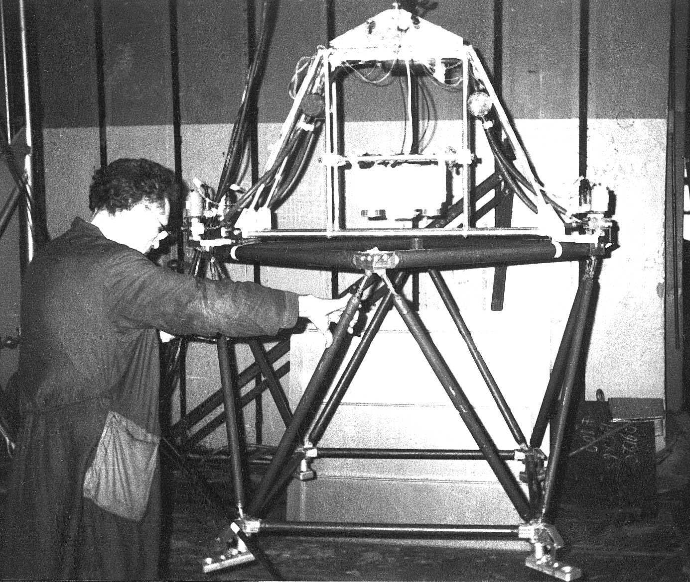
The platform is supplied with four pulse engines. The engine is the electric-magnetic valve where the power is produced by escaping the compressed air. The balloon with compressed air is placed aside in the test hole and connected with engines by pneumatics lines. The power of each engine ~ 2.5 N. Position-sensitive detector and on-board computer is places at the platform. Two marked beacons are displaced on the floor near the setting place. The platform performs the motion control along two translational axes in horizontal plane and angular attitude about vertical axis. The on-board computer used the approach and docking control algorithm similar to that was described in paragraph 3. During the experiments an accurate of matching the assembly points of the load and the support was in the range  0.6 sm

This technological model is elaborates by specialists from the Space Research Institute in close cooperation with participators of a given project.

Results of computer simulations and experimental tests with the platform prototype confirm the following conclusions:

• The proposed methods of flight control are able to perform the safety and accurate Automated Module operating in Space.

• Declared properties of the Module are quite reliable;

• There are no technical obstacles in the device creation.

( LES HALLES) ESPACE D’ART CONTEMPORAIN RUE PIERREPÉQUIGNAT 9
(ABOVE SPACE IS RESERVED FOR RECORDING INFORMATION) MINNESOTA WETLAND
0B0703 TRAFFIC NOISE IN GREEN AND OPEN SPACES (EDITION

Tags: automated module., accurate automated, automated, methods, trajectory, docking, module, space, based

---

• 13 MUSTERBV BETRIEBSVEREINBARUNG ZUR BESSEREN VEREINBARKEIT VON BERUF UND
• 34 FIRMSPECIFIC COMPETENCIES DETERMINING TECHNOLOGICAL INNOVATION A SURVEY IN
• EXECUTIVE SUMMARY LAPORAN KUNJUNGAN KERJA KOMISI I DPR RI
• ACADEMIC WRITING TIP 26 THE APOSTROPHE HERE ARE A
• FORM ICB RESEARCH DEGREE REGISTRATION AMENDMENT FORM PLEASE READ
• „A PTE UTAZÓ NAGYKÖVETE” TÁMOGATÁSI PROGRAM PÁLYÁZATI FELHÍVÁS 2019
• DOMINO DEMUESTRA LA VERSATILIDAD Y EL VALOR AÑADIDO DE
• SEXTO SOCIALES DISEÑO GRAFICO TEMARIO PARA EXAMEN DEL
• ZASADY EDYTORSKIE PRZYGOTOWANIA PRACY MAGISTERSKIEJ NA WYDZIALE WYCHOWANIA FIZYCZNEGO
• PRESENTACIÓN DE LA NUEVA TINTA NEGRA 950BK 100 LIBRE
• CHAPTER 3 FILLING VACANT POSITIONS APPENDIX 3C WHAT
• DOMINO AMPLÍA SU OFERTA DE SOLUCIONES DE INYECCIÓN DE
• 8VA BIENAL DEL COLOQUIO DE TRANSFORMACIONES TERRITORIALES AUGM MESA
• 2SOMHI SOL MI DO RE7 UN NOU DIA ES
• 1) FOR A POPULATION THAT HAS A STANDARD DEVIATION
• DEPARTMENT OF DEFENSE (DOD) ENTERPRISE SOFTWARE INITIATIVE (ESI) 2003
• LIST OF AGENCIES WITH ELECTED OFFICIALS REQUIRED FOR POLITICAL
• POWERPLUSWATERMARKOBJECT98827025 SFA NAME SFA ADDRESS SFA CONTACT INFORMATION CALL
• DOMINO LANCEERT NIEUWE RANGE VAN VEELZIJDIGE ZWARTE INKTEN VOOR
• EL IOBA INVESTIGA CÓMO AUMENTAR LA AGUDEZA VISUAL CON
• BILATERAL TREATIES OF THE REPUBLIC OF BELARUS ON LEGAL
• M ODELO DE DECLARACIÓN RESPONSABLE DOC 2 RELATIVA A
• ORDEN DE 25 DE SEPTIEMBRE DE 2000 DE LA
• FOCUS GROUP INSTRUCTIONAL GUIDELINES FROM AN INSTITUTIONAL REVIEW BOARD
• SECRETARÍA DE EDUCACIÓN JALISCO SUBSECRETARÍA DE EDUCACIÓN MEDIA SUPERIOR
• ENGLISH 7 ANTICIPATION GUIDE FOR DRAMA ELEMENT NOTES NAME
• DOMINO ELEVA EL LISTÓN EN INTERPACK 2014 COMUNICADO DE
• A YUNTAMIENTO DE MURCIA SERVICIO DE DEPORTES AVENIDA DEL
• AKER SYKEHUS NEDENSTÅENDE ER MENT Å SKULLE GI SVAR
• QUEBEC HALL LTD (HOME FOR RETIRED CHRISTIANS) CONFIDENTIAL APPLICATION

• Normas Técnicas Complementarias Para Diseño y Construcción de Cimentaciones
• “SYSTEM ACCREDITATION AN INNOVATIVE APPROACH TO QUALITY ASSURANCE AND
• REGULAMIN ORGANIZACYJNY URZĘDU GMINY JAROSŁAW ROZDZIAŁ I POSTANOWIENIA OGÓLNE
• À REA DE PRESIDÈNCIA DIRECCIÓ DE RELACIONS INTERNACIONALS DESEMBRE
• UNIVERSIDAD DE COLIMA FACULTAD DE MEDICINA VETERINARIA Y ZOOTECNIA
• ORGANISMO INDIPENDENTE DI VALUTAZIONE DELLA PERFORMANCE DELL’AZIENDA OSPEDALIERA PER
• SUMANI EKONOMIKA PRIORITETAS TIKSLAI UŽDAVINIAI RODIKLIAI Į AUKŠTĄ PRIDĖTINĘ
• CONTRATO DE AGENCIA NO20 REUNIDOS DE UNA PARTE
• CONTACT NORMAN BLACK 4048287593 UPS APPLAUDS POSITIVE MOVEMENT OF
• BALLOON TRACK – STRUČNÝ NÁVOD PRO INSTALACI A NASTAVENÍ
• RIJEKA 16 PROSINCA 2008 INFORMACIJA ZA MEDIJE PRIMANJE ZA
• MICHAEL JACKSON WWWFAMOUS PEOPLE LESSONSCOM MICHAEL JACKSON HTTPWWWFAMOUSPEOPLELESSONSCOMMMICHAELJACKSONHTML CONTENTS
• Nerc Style Guide as of March 31 2005 Blackstart
• NA PODLAGI 5 ČLENA STATUTA OBČINE STRAŽA (URADNI LIST
• 20202021 NAAE STATE OFFICER ROSTER PLEASE COMPLETE THIS FORM
• 1 RESEARCH ACTIVITY (MAX 1000 WORDS) THE STUDY OF
• LISTADO DE LIBROS “CITA A CIEGAS CON UN LIBRO”
• JURNAL PENGARUH FAKTOR MOTIVASI INTERAKSI SOSIAL MOTIVASI DOKUMENTASI MOTIVASI
• Zánka Község Önkormányzat Képviselőtestülete 392009 (xii15) Rendelete Zánka Község
• MANUAL DE USUARIO MOTOR SOLICITUDES VERSIÓN 5 – OCTUBRE