MODELLING THE VERTICAL MOVEMENTS OF THE EARTHS CRUST WITH

11 KARIN KNOTTENBAUER – MODELLING INNOVATION AND STRUCTURAL CHANGE
19TH EUROPEAN CONFERENCE ON MODELLING AND SIMULATION ‘SIMULATION IN
2006BASED PUPIL PROJECTIONS METHODOLOGY 1 THE MODELLING PROCESS USES

28 POSITIVE AND NEGATIVE PEER MODELLING EFFECTS ON YOUNG
34 PROTEOMIC REMODELLING OF PROTEASOME IN RIGHT HEART FAILURE
5 MODELLING INTONATIONAL VARIATION IN ENGLISHTHE IVIE SYSTEM MODELLING

Modelling the vertical movements of the earth's crust with the help of the collocation method

MODELLING THE VERTICAL MOVEMENTS OF THE EARTH'S CRUST WITH THE HELP OF THE COLLOCATION METHOD

Kamil Kowalczyk

University of Warmia and Mazury in Olsztyn

[email protected]

ABSTRACT

In 2003, the fourth levelling campaign was completed in Poland. This campaign, together with the previous one carried out in 1974-1982, gave a very good opportunity to determine the land uplift in the area of Poland. The paper describes shortly the third and fourth campaigns, the computation of the relative land uplift, computation of land uplift referred to the mean sea level and modelling the land uplift by the least square collocation method. The obtained results were compared with the computation done by the Institute of Geodesy and Cartography in 1986.

1.1 Introduction

Work is in progress at present in Europe on the realization of the second stage of unifying the levelling networks in Europe, i.e. the kinematic adjustment of the UELN-95 network (resolution 5 of the EUREF symposium, Prague 1999). To perform such an adjustment, a model is necessary for vertical crustal movements for the area of Europe.

Such a model for the area of Poland has been created (Kowalczyk, 2006) with the use of levelling data (the precise levelling campaign 1974-1982; 1999-2003) and mareographic data. The collocation method was used to create this model. This method is commonly used for interpolation of the intervals between the geoid and ellipsoid. Markov’s and Hirvonen’s covariance functions were utilized as analytical covariance functions.

During work on determining vertical movements at nodal bench marks, 235 common nodal bench marks were identified in both campaigns and 360 common levelling lines out of the total number of 382.

Relative vertical movements at the nodal bench marks were determined in relation to the nodal bench mark in Władysławowo. The “observed” vertical movements at these bench marks were determined in relation to the mareograph in Władysławowo, assuming the mareograph’s vertical movement as the mean vertical movement from four mareographic stations, i.e. Świnoujście, Kołobrzeg, Ustka, Władysławowo. The figure below presents the observed vertical movements in the area of Poland.

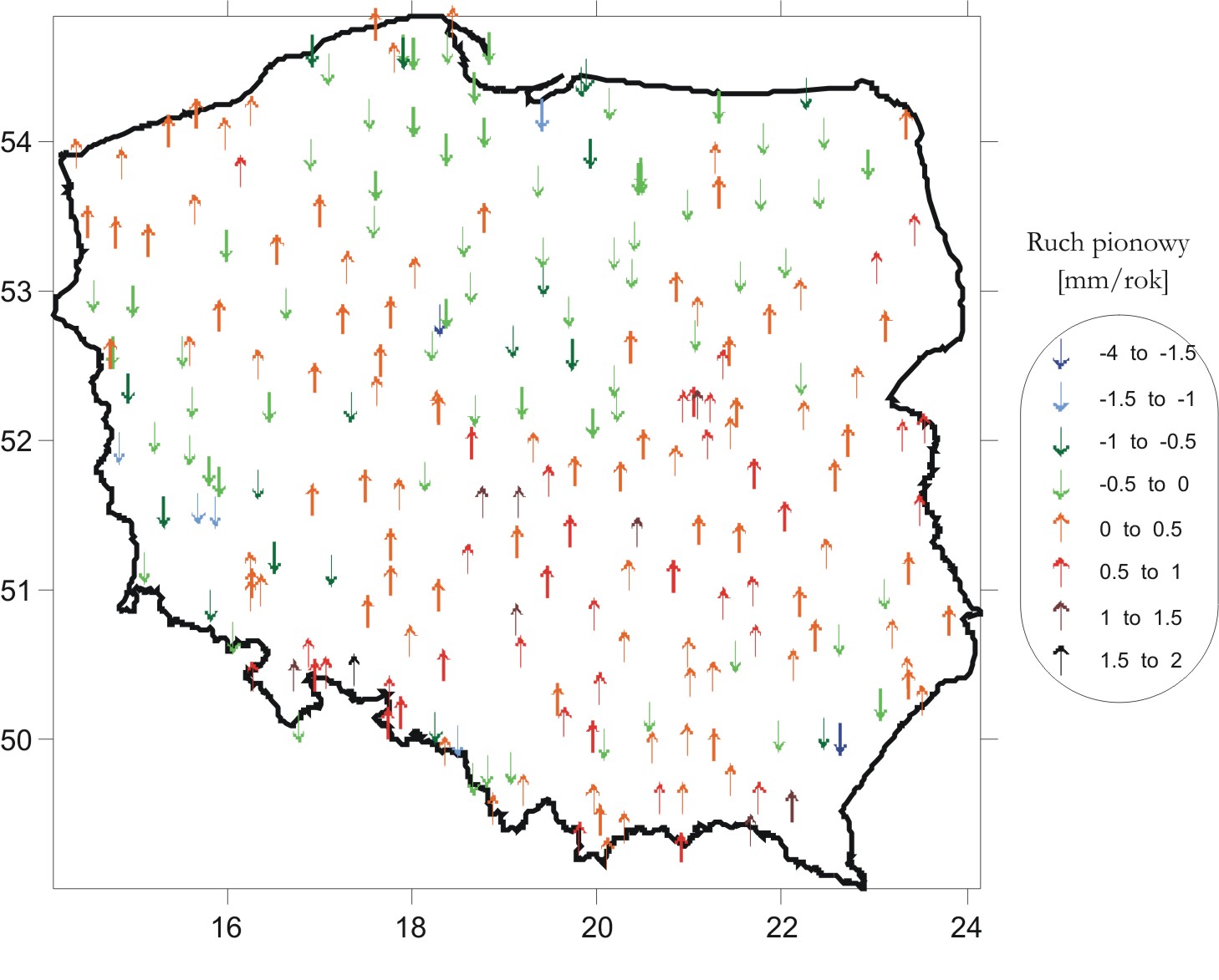
MODELLING THE VERTICAL MOVEMENTS OF THE EARTHS CRUST WITH

Fig. 1. The observed vertical movements in the area of Poland

Unfortunately, on account of the bench marks’ distribution (they do not cover evenly and densely enough the whole area of the country), the obtained model had to be condensed, using for this purpose interpolation and extrapolation of vertical movements.

There are many methods of interpolation using functions defined by means of a diagram, a table, or an analytical expression (Waliszewski, 1990), however, the irregular character of vertical movements makes their determination impossible by means of an exact analytical formula. This is why a mathematical model should be used for the interpolation of vertical movements.

In the case of such type of data (irregular), the stochastic model is the best (Jasecki 1983). From the literature (Moritz, 1973; Hardy, 1984; Leonhard, Niemeier, 1986; Jasecki, 1983) it appears that the most proper interpolation method for creating a numerical model of vertical movements is the collocation method.

1.2 Bases of interpolation by the least square collocation method

The collocation method proposed by Krrarup in the 1950s, spread by Moritz, has found broad use primarily in physical geodesy, but it can be successfully used in other fields of geodesy, among others, for the interpolation of vertical crustal movements. The theoretical bases of this method presented in this paper were developed on the basis of information provided in the literature (Heiskanen, Moritz, 1967; Moritz, 1980). This method can be presented in outline in the following way. The covariance of observations is called the mean value of the product of two observations at points separated by a constant distance .

If we have at our disposal observations of the network bench marks’ vertical movements, then we calculate the interpolated vertical movement in the point from the formula:

(1)

where:

– vector of the nodal bench marks’ vertical movements,

– vector of the covariance between and ,

MODELLING THE VERTICAL MOVEMENTS OF THE EARTHS CRUST WITH – matrix of the covariance between observations .

The accuracy of interpolation measured by the mean error amounts to:

MODELLING THE VERTICAL MOVEMENTS OF THE EARTHS CRUST WITH (2)

The problem of interpolation, mentioned above, can be solved only in the case when we know covariance functions. Then all elements of the matrix C and the vector C_Pcan be calculated. To pass on to the covariance function, one should first define the covariance itself.

Let’s assume that we are dealing with a set of quantities (observations) distributed in a certain area, whose sum equals zero. If these quantities can be considered a function of the position, then the integral over the given area should equal zero (Heiskanen, Moritz, 1967). Such a set is the set of values of vertical movements in the area of the whole Earth.

The covariance of vertical movements can be defined as the mean value of the product of vertical movements , in the whole examined area at points and , separated by the segment .

In the case of small values of d, e.g. 1 km, almost equals , that is to say covariance almost equals variance. In other words, there is a strong correlation between and . The covariance decreases together with an increase in d, because vertical movements become more and more independent. In the case of very great distances d, the covariance will be very small, but never equal to zero, for vertical movements are caused not only by local changes in Earth’s crust, but also by regional factors.

For the needs of interpolation the terrestrial globe can be defined locally as a plane. Let’s assume that (x, y) define coordinates on a plane and that the points P( , ) and Q( , ) lie on this plane. Then, homogeneity and isotropy show that the covariance function can depend only on the distance between the points PQ:

(3)

It is then possible to express the covariance function by the analytical expression (Heiskanen, Moritz, 1967)

(4)

where: , , and  coefficients determined by Hirvonen. They amount to: C_o = 337 mGal², B^-1 = 40 km, m = 1 (Heiskanen, Moritz, 1967).

Other proposals of analytical covariance functions can be found, among others, in Moritz’s paper (1978). In the quoted paper, the author provides the following analytical expressions as:

(5)

and other possible analytical expressions derived from Markov’s model:

(6)

The following expressions are called Markov’s models of higher orders:

(7)

(8)

More information on these models can be found in papers by Jordan (1972), Kasper (1971) and Shaw et al., (1969).

The coefficients A, B, D from the formulas (4 – 8) can be determined from the empirical values of the covariance function. Basing oneself on the formula for calculating the empirical covariance function for mean gravimetric anomalies (Tscherning, Rapp, 1974), one can write a practical formula for also calculating the empirical covariance function for vertical movements, i.e.:

i, j =1, 2, 3….n (9)

where: n – the number of points at which vertical movements were determined, d – the distance between these points.

In the present paper, the program empcov from the GRAVSOFT package was used for calculations (Tscherning et al., 1992)

1.3 Determination of the empirical covariance function of the “observed” vertical crustal movements in the area of Poland

To determine the empirical covariance function on a representative group of points nodal bench marks of a network of vertical movements were assumed. The variance was given in , the correlation distance in degrees of the arc.

The calculations yielded the following values of parameters of the empirical covariance function determined on the basis of the nodal bench marks: variance - 0.2928, 1/2 - 0.1464, correlation distance - 0.3652.

The figure (Fig. 2) below presents the diagram of the empirical covariance function and diagrams of Markov’s and Hirvonen’s analytical function.

MODELLING THE VERTICAL MOVEMENTS OF THE EARTHS CRUST WITH

Fig. 2. Diagram of the empirical covariance function calculated on the basis of nodal bench marks

As shown Hirvonen’s analytical function is better matched to the empirical function.

1.4 Model of vertical crustal movements in the area of Poland

The realisation of the interpolation required the preparation of appropriate data, on which the calculations were performed. The intersections of meridians and parallels in the area of Poland were assumed as interpolated points in intervals of 20’x20’.

To avoid the formation of a singular matrix, using Matlab’s authoring scripts, it was attempted to define the optimum area on whose basis the vertical movement would be determined on such defined grid. On their basis and after several tests the optimum area was defined by a 50 km long radius.

The observed vertical movements at the nodal bench marks were assumed as points of departure for interpolation with values determined in relation to the nodal benchmark in Władysławowo connected with the mareographic station in Władysławowo. The interpolation was performed with the use of own scripts written in the Matlab program. These programs, named “markow” and “hirvonen”, serve for interpolation by the method of collocation with the use of appropriate covariance functions and calculating the interpolation’s mean error.

Before starting calculations, tests of the programs were carried out on about 10% of the nodal bench marks. They consisted in calculating, by means of both models (Markov’s and Hirvonen’s), the relative vertical movements at selected nodal bench marks and comparing them with the relative vertical movements obtained from the adjustment of the network by the parametric method.

The graphical expression of the obtained results is presented in Fig. .3

MODELLING THE VERTICAL MOVEMENTS OF THE EARTHS CRUST WITH

Fig. 3 Comparison of vertical movements

1.5 Model of the “observed” vertical crustal movements in the area

of Poland

On the basis of the procedure and formulas presented above, the following models of vertical crustal movements in the area of Poland were created.

Model of vertical movements with the use of Markov’s analytical function and Hirvonen’s analytical function (Fig. 4).

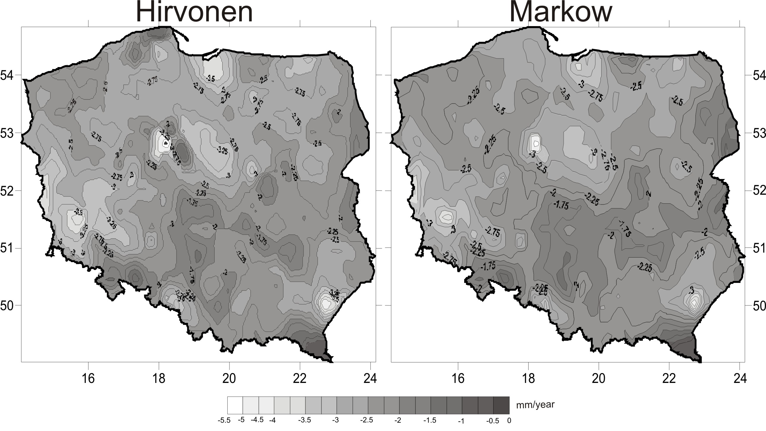
MODELLING THE VERTICAL MOVEMENTS OF THE EARTHS CRUST WITH

Fig. 4. Model of the observed vertical movements determined with the use of Markov’s and Hirvonen’s analytical function

The mean error of interpolation of vertical movements by the collocation method was also determined with the use of Markov’s analytical function. It is contained within the range from 0 to 0.30 mm/year (Fig. 5).

MODELLING THE VERTICAL MOVEMENTS OF THE EARTHS CRUST WITH

Fig. 5. The mean error of interpolation by the collocation method with the use of Markov’s analytical function

The mean error of interpolation of vertical movements by the collocation method was determined, similarly as above, with the use of Hirvonen’s analytical function. It is contained in the bounds from 0 to 0.25 mm/year (Fig. 6).

In comparing models obtained by means of Markov’s and Hirvonen’s functions, it can be seen that mean vertical movements do not differ greatly. The differentiation is greatest near Inowrocław and near Gdańsk. In the remaining area of the country, the values of vertical movements are close to one another, and the course of isolines is similar. The mean error of interpolation by the collocation method is, in both cases, within the range from 0 to 0.30 mm/year. A smaller mean error occurs in the greater part of Poland in the case of using Hirvonen’s function – from 0 to 0.15 mm/year. In the model in which Markov’s function was used, a mean error with the value from 0.1 to 0.2 mm/year dominates.

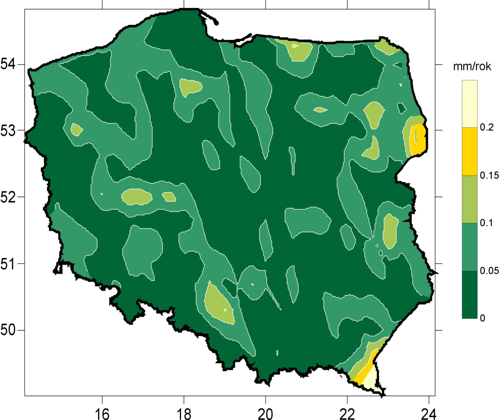
MODELLING THE VERTICAL MOVEMENTS OF THE EARTHS CRUST WITH

Fig. 6. The mean error of interpolation by the collocation method with the use of Hirvonen’s analytical function

1.6 Summary and conclusions

The collocation method is suitable for interpolation of vertical movements.

Better results were obtained with the use of Hirvonen’s analytical function.

A model was created of contemporary vertical crustal movements in the area of Poland with the use of interpolation by the collocation method.

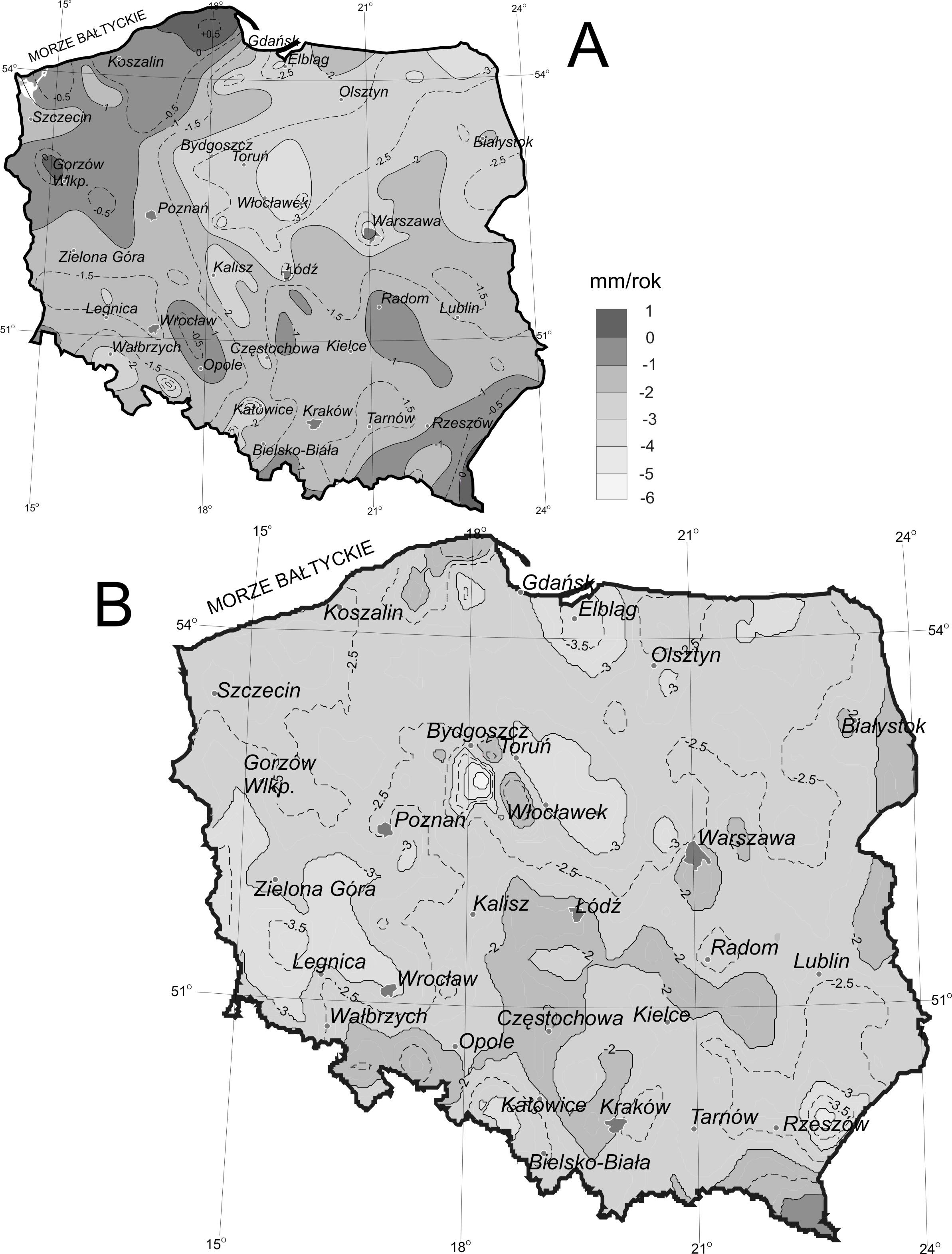
Fig. 7. Vertical crustal movements in the area of Poland

The model was created in two variants: as a numerical set of interpolated vertical movements at points of the grid of meridians and parallels and an analogue map of vertical crustal movements in the area of Poland.

On the basis of the numerical model, the possibility exists of interpolating vertical movements anywhere in Poland. The first tests carried out by Prof. Adam Łyszkowicz confirmed the model’s accuracy, which, in consequence, also confirmed the possibility of using collocation for elaborating vertical crustal movements.

1.7 Literature

Hardy R.L. 1984, Kriging, collocation and biharmonic models for applications in earth sciences. Tech. Papers of the American Congress on Surveying and Mapping, pp.363-372.

Heiskanen W., Moritz H., 1967, Physical Geodesy, W.H. Freeman and Company, San Francisco and London.

Jasecki M., 1983, The covariance function in the process of developing geodetic data, Geodesy and Cartography, PWN, 32(4): 283-292, Warsaw.

Jordan S. K., 1972. Self-Consistent statistical model for the gravity anomaly, vertical deflections, and undulation of the geoid. J. Geophys. Res., 77(20): 3660 3670.

Kasper J. F., 1971. A second-order Markov gravity anomaly model, J. G. Res., 76(32): 7844 7849.

Leonhard Th., Niemeier W. (in Eds. H. Pelzer and W. Niemeier), 1986, A kinematic model to determine vertical movements and its application to the testnet Pfungstadt. Contributed paper to the Symp. on height determination and recent vertical crustal movements in Western Europe, held at the Univ. Hannover. Sept. 15-19, 1986, Dummiers Verlag-Bonn.

Moritz H., 1978, Least-squares collocation. Rev. Geoph Space Physics, 16(3).

Moritz H., 1980, Advanced physical geodesy. H. Wichmann Verl. , Karlsruhe.

Tscherning C.C., Rapp R.H., 1974, Closed Covariance Expressions for Gravity Anomalies, Geoid Undulations, and Deflections of the Vertical Implied by Anomaly Degree-Variance Models. Rep. of the Dep. of Geod. Sci. No. 208, The Ohio State University, Columbus.

Tscherning C., Forsberg R., Knudsen P., 1992, The GRAVSOFT package for geoid determination. First Continental Workshop on the Geoid in Europe Towards a Precise Pan.

Kowalczyk K., 2006, Determination of a model of vertical crustal movements in the area of Poland, Doctoral thesis, UWM Olsztyn.

The paper was realized within centres on science in summers 2005/2006 work.

7 MATHEMATICAL MODELLING WORKSHEET 14 TRAFFIC FLOWS AND PEDESTRIAN
7 MATHEMATICAL MODELLING WORKSHEET 8 MODELS OF A COMPETITIVE
7 MODELLING COPPER (II) LIQUIDLIQUID EXTRACTION THE SYSTEM ACORGA

Tags: crust with, vertical, movements, earths, crust, modelling