BIOMETRY (BIOL40906090) FALL 2018 HOMEWORK 4 STUDENT NAME
BIOMETRY (BIOL40906090) FALL 2018 HOMEWORK 4 STUDENT NAMEWNIOSKI O WYDANIE PASZPORTÓW BIOMETRYCZNYCH MOŻNA SKŁADAĆ ORAZ ODBIERAĆ
Biometry (Biol4090-6090) - Fall 2018 Homework #4 Student name: ______KEY__________
NOTE: Do not Turn This In. Homeworks will not be graded
Homework in preparation for quiz #4 – on October 4th
Use R exercises to develop your computer skills.
1) Explain the following terms using the words provided in parenthesis (+0.25, each):
-Parametric statistics (normality) = Built upon the assumption that the observations (data) come from a normal distribution, and make inferences about the specific parameter of that distribution
- Non-parametric statistics (distribution-free) = A type of distribution-free techniques do not rely on any assumptions concerning the distributions of the observations (data). Two examples of distribution-free statistics involve randomization tests, comparing observed and expected patterns for shuffled data, and non-parametric statistical tests, using ranked data to compare the medians, rather than the means.
- Q-Q plot (quantiles) = The quantile-quantile (q-q) plot is a graphical technique for determining if two data sets come from populations with a common distribution. A q-q plot is a plot of the quantiles of the first data set against the quantiles of the second data set. If all the data points fall on the diagonal of the plot, then the variable is normally distributed. Any points that do not follow the diagonal show deviations from normality.
- Shapiro - Wilks (S-W) test (normality) = A statistical test developed to determine whether a given frequency distribution originated from a normally distributed population, with the same mean parameters as the sample (mean, S.D.). The null hypothesis is that the sample came from the normal distribution. A significant result suggests that the sample is not normally distributed.
2) Highlight the differences amongst the different tests used to assess data normality, by filling in the blanks below with one of the five possible answers: “S-W test”, “Levene’s Test”, “none” or “all of the above” (each is 0.10 points):
- compares observed data distribution against a normal distribution with same mean and S.D.: S-W
- compares the variances of two observed data distributions against each other: Levene’s Test
- compares the variance of one observed data distribution against the variance of a normal distribution with same mean and S.D.: NONE
- assumes the data follow a normal distribution: Levene’s Test
- assume the data were collected using random sampling: ALL OF THE ABOVE
- null hypothesis for this test states that the observed data and the theoretical distribution are the same (the observations come from the same theoretical biological population): 1-sample K-S test
3) Open the file Hw4Data.xlss with R and use these observations, drawn from three random variable distributions (all derived from theoretical distributions with a mean = 10 and a variance =10) for the following exercise.
Create a frequency table for these three datasets of 100 data points each and use this information to fill in the table below (+0.05 each entry). Note – because these are random samples from theoretical distributions , the parameter estimates (x-bar, S.D.) will vary from the real parameters ( µ, σ).
|
mean sd 5% 50% 95% n distribution_1 9.724613 2.943354 5.348738 9.644506 15.74372 100 distribution_2 9.720000 3.048696 5.000000 10.000000 14.05000 100 distribution_3 9.705097 3.033430 5.113512 9.761769 14.40838 100
|
|
|
|
|
|
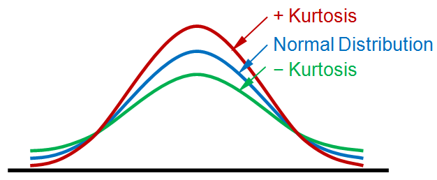
For each distribution, calculate the skewness (and the SE), calculate the kurtosis (and the SE), create a histogram, create a box plot of each distribution.
For reference: check out this diagram:
Paste the information below (+0.25 for each distribution):
Distribution_1:
Skewness: 0.60643213
Skew.2SE: 1.25617841(skew divided by 2 * SE)
Interpret this skewness: Looks very symmetrical, but it has positive skewness, suggesting that the right tail (on the positive side) is longer and that the mass of the distribution (the observations) is concentrated disproportionately on the left side of the figure (on the negative side). The long tail is balanced by more observations on the left. Note: however, skew is significant (the skew * 2 SE value is > 1)
Kurtosis: 0.66793461
Kurtosis.2SE: 0.69819270 (kurtosis divided by 2 * SE)
Interpret this kurtosis: Distribution has positive kurtosis (leptokurtic), meaning that the distribution is “slender”, has a taller and skinnier peak around the mean (more observations around the mean) and fewer observations on the tails than expected, as indicated by the positive kurtosis. Note: however, kurtosis is not significant (the kurtosis * 2 SE value is < 1)
P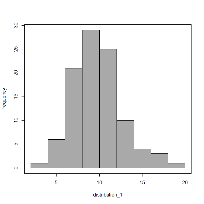
 aste
Histogram and Box Plot:
aste
Histogram and Box Plot:
Briefly explain and discuss, whether this distribution looks like a normal distribution, based on the skewness / kurtosis and the shape of the histogram? Explain why / why not:
Looks like a normal distribution, but it is not, as evidenced by the results of the W-S test (normtest.W = 0.96997046,normtest.p = 0.02198988), since the p value < 0.05. While the skewness surpasses the “rule of thumb” threshold (skew.2SE> 1), the kurtosis is less than the “rule of thumb” threshold (kurtosis.2SE> 1). Overall, this is enough to cause a lack of normality.
Distribution_2:
Skewness: 0.1747337
Skew.2SE: 0.3619477(skew divided by 2 * SE)
Interpret this skewness: Looks very symmetrical, but it has a slightly positive skewness, suggesting that the right tail is longer, and the mass of the distribution is shifted on the left of the figure. Note: however, skew is not significant (the skew * 2 SE value is < 1)
Kurtosis: 0.2190700
Kurtosis.2SE: 0.2289941 (kurtosis divided by 2 * SE)
Interpret this kurtosis: Distribution is slightly positive (leptokurtic), meaning that the distribution has a taller and skinnier peak right on the mean (more observations closer to the mean than expected). Note: however, kurtosis is not significant (the kurtosis * 2 SE value is < 1)
P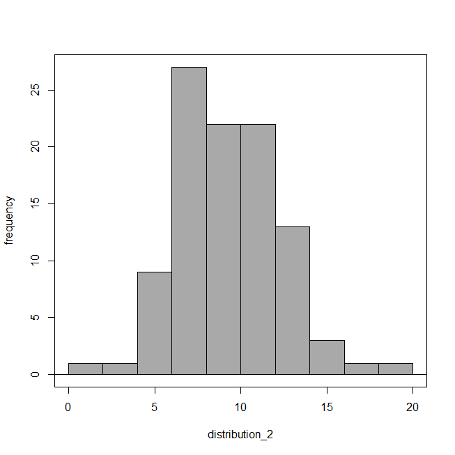
 aste
Histogram and Box Plot:
aste
Histogram and Box Plot:
Briefly explain and discuss, whether this distribution looks like a normal distribution, based on the skewness / kurtosis and the shape of the histogram? Explain why / why not:
Looks like a normal distribution, as evidenced by the results of the W-S test (normtest.W = 0.9808325, normtest.p = 0.1542661). since the p value < 0.05. Neither the skewness nor the kurtosis surpass the “rule of thumb” thresholds (skew.2SE> 1 and kurtosis.2SE> 1). Overall, this is a normally distributed dataset.
Distribution_3:
Skewness: -0.07998707
Skew.2SE: -0.16568719 (skew divided by 2 * SE)
Interpret this skewness: Looks very symmetrical, but it has a slightly negative skewness, suggesting that the left tail is longer, and the mass of the distribution is shifted on the right of the figure. Note: however, skew is not significant (the skew * 2 SE value is < 1)
Kurtosis: -0.20686772
Kurtosis.2SE: -0.21623903 (kurtosis divided by 2 * SE)
Interpret this kurtosis: Distribution is slightly negative (platykurtic), meaning that the distribution has a flatter distribution (with fewer observations near the mean) than expected. thresholds (skew.2SE> 1 and kurtosis.2SE> 1). Overall, this is a normally distributed dataset.
Paste Histogram and Box Plot:
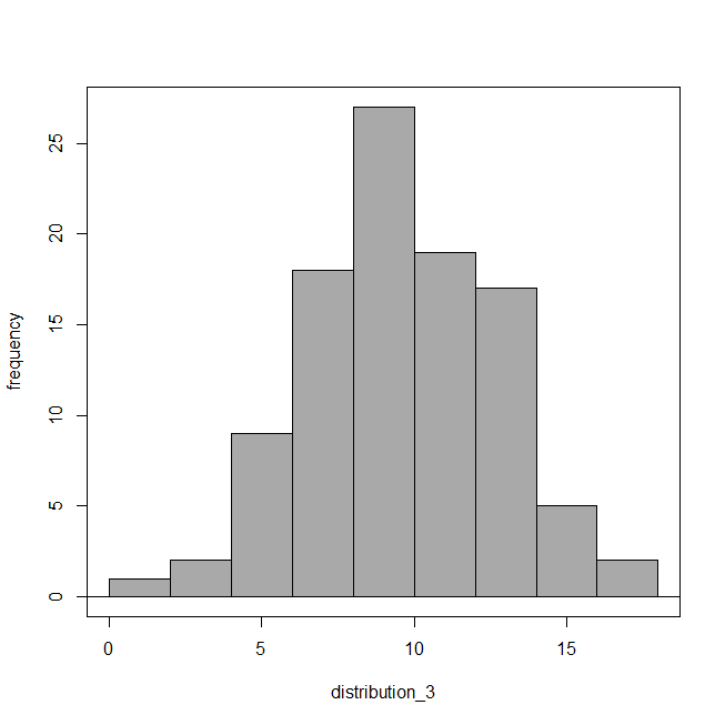
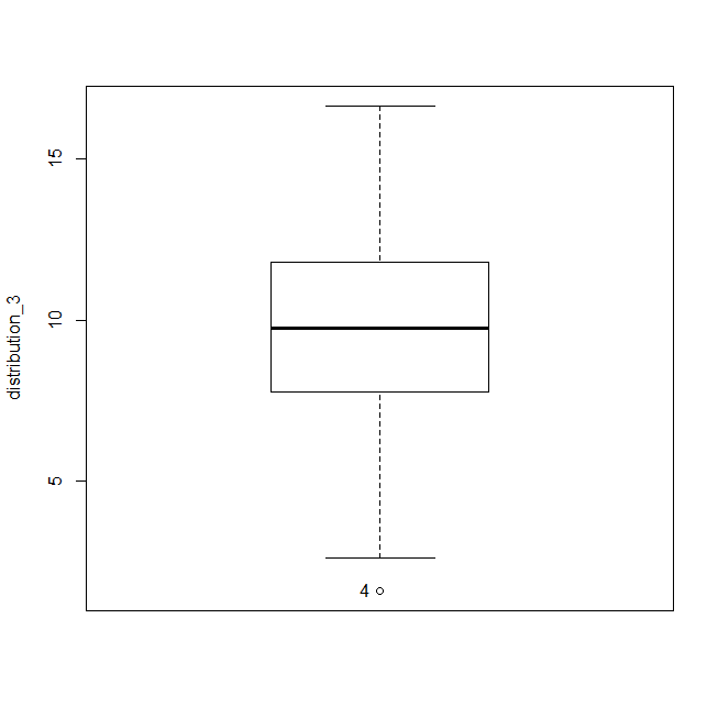
Briefly explain and discuss, whether this distribution looks like a normal distribution, based on the skewness / kurtosis and the shape of the histogram? Explain why / why not:
Looks like a normal distribution, as evidenced by the results of the W-S test (normtest.W = 0.99475079, normtest.p = 0.96818667). since the p value < 0.05. Neither the skewness nor the kurtosis surpass the “rule of thumb” thresholds (skew.2SE> 1 and kurtosis.2SE> 1). Overall, this is a normally distributed dataset.
4) Compare each distribution to a normal distribution with the same mean / S.D. (use parameters estimated in question #2, above (+0.50 for each distribution):
Distribution_1:
Paste results table here, and interpret the S-W test result:
was this result significant: (Y / N), why? Yes, p = 0.022 is < 0.05
is distribution 1 normally distributed: (Y / N), why? No – because the null was rejected
using the Q-Q plot, are there more observations than expected in the tails or on the center of mass of the observed distribution? Does this agree with the sign (+/-) of the kurtosis of this distribution you calculated in question #3? Why / why not?
Paste the detrended normal Q-Q plot here – for reference:
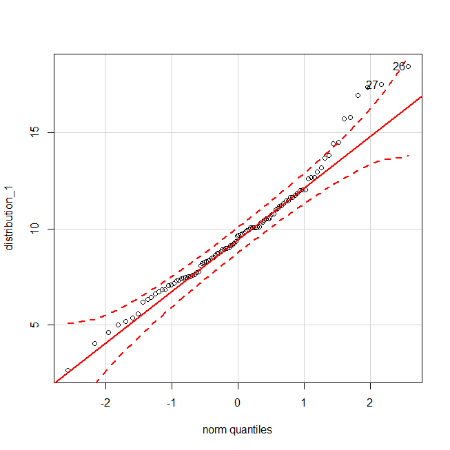
The Q-Q plot agrees with the answer in question 3 because it shows an excess of observations (positive values) from the two tails of the distribution (the smallest and the largest values), with a larger deviation for the largest values (around quantile 2). This suggests that the observed distribution has less observations in the center (leptokurtic). The asymmetry of the deviations around the mean, with smaller left deviations (smaller values), suggests that the distribution has a positive skew, with a longer right tail and more excess observations to the right.
Distribution_2:
Paste results table here, and interpret the S-W test result:
was this result significant: (Y / N), why? No, p = 0.154 is > 0.05
is distribution 2 normally distributed: (Y / N), why? Yes - because the null was not rejected
using the Q-Q plot, are there more observations than expected in the tails or on the center of mass of the observed distribution? Does this agree with the sign (+/-) of the kurtosis of this distribution you calculated in question #3? Why / why not?
P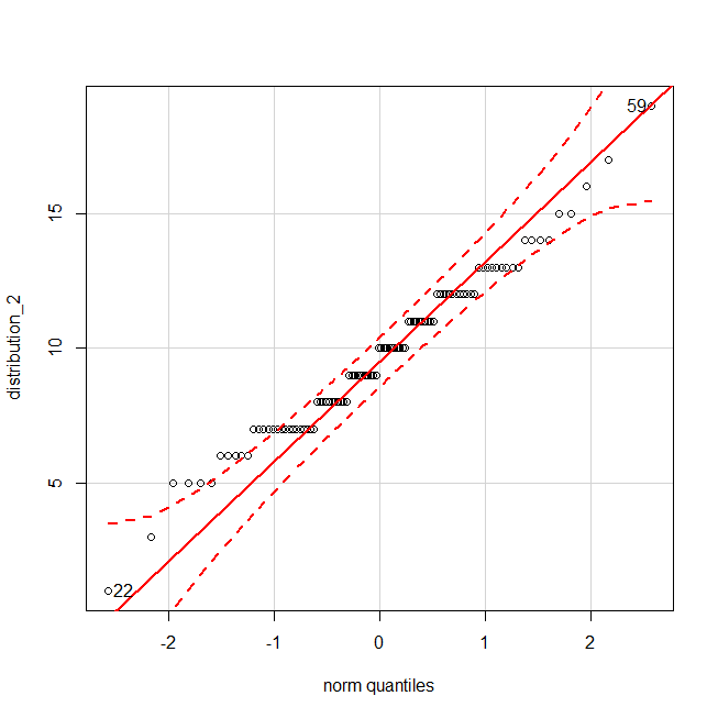 aste
the detrended normal Q-Q plot here – for reference:
aste
the detrended normal Q-Q plot here – for reference:
This Q-Q plot agrees with the answers in question 3. Because it shows an excess of observations (smallest values) from left tail of the distribution and a deficit of values (largest values) in the right tail of the distribution. The asymmetry of the deviations about the normal distribution suggests that the distribution has a left skew (positive skew) with a longer right tail.
Distribution_3:
Paste results table here, and interpret the S-W test result:
was this result significant: (Y / N), why? No, p = 0.968 is > 0.05
using the Q-Q plot, are there more observations than expected in the tails or on the center of mass of the observed distribution? Does this agree with the sign (+/-) of the kurtosis of this distribution you calculated in question #3? Why / why not?
Paste the Normal Q-Q plot here (not the detrended plot) – for reference:
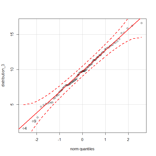
This Q-Q plot agrees with the answers in question 3, since the skewness is less clear, because the Q-Q plot shows a scatter of positive and negative points, with an excess of observations (positive values) along the right tail of the distribution (the larger values), and a deficit of values (negative values) in the left tail. This suggests that the skewness is very small, since large asymmetries in the distribution are not clearly visible. Similarly, the kurtosis is also hard to evaluate visually, since the positive and negative deviations are spread throughout the range of observed values. These graphs reinforce the notion that the skew and kurtosis quantified in question 3 are very small.
5) Given that distribution_1 was log normal, distribution_2 was Poisson, and distribution_3 was normal, answer the following questions (+0.25 each). Note: Re-read the notes from lecture 5:
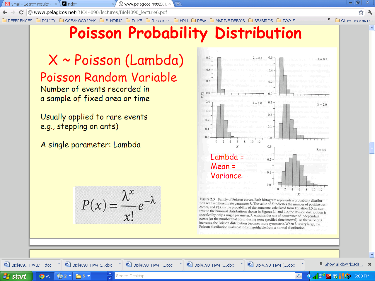
- What is the only parameter of the Poisson distribution (Lambda) and what does it quantify?
The Poisson distribution only has one parameter (Lambda), which quantified its mean and the variance.
In the Poisson distribution, the mean = the variance.
- Briefly describe how the shape of the Poisson distribution changes as the parameter Lambda increases from 0.1 to 10 (range of values from lecture and this example)? Specifically, describe what happens to the skewness and the kurtosis of the distribution.
The Poisson distribution changes shape as lambda increases from a value of 0.1 to a value of 10 (the current value in this example). Please consult the following figure from your class notes (taken from the Gotelli book), showing that the distribution starts as being highly asymmetrical, and then becomes increasingly symmetrical. Thus, the skewness ranges from a large positive value (when Lambda = 0.1) to a very small positive value (when Lambda = 10). Please check out this slide from lecture 9.
Tags: (biol40906090), homework, biometry, student
- KEAN UNIVERSITY UNION NEW JERSEY FALL 2009 THE MULTICULTURAL
- REVISED 604 AGRICULTURAL DISTRICT RECERTIFICATION SURVEY DATE DEAR
- HOJA DE VIDA ING SANTIAGO EDUARDO ANTOGNOLLI
- 523 dm 1 Page 5 of 5 Department of
- Mieterschutzbund Berlin ev Presseerklärung 1492012 Nachbar Zahlt Weniger
- DEFINING PROJECT RESULTS A GUIDE FOR APPLICANTS PROJECT RESULTS
- DWU WATER AND WASTEWATER PROCEDURES AND DESIGN MANUAL D
- Short Form of the Informant Questionnaire on Cognitive Decline
- STANDARD OPERATING PROCEDURE (SOP) FOR DEAD OR SEVERELY INJURED
- JAMES RENNIE BEQUEST REPORT ON EXPEDITIONPROJECTCONFERENCE PROJECT HOW DO
- CENSUS 2000 SUMMARY FILE 1 DATA FOR NEW JERSEY
- NIEUWSBERICHT HYUNDAI LANCEERT NVIDIA DRIVE EEN INFOTAINMENT EN AIPLATFORM
- 4 REVIDERAD UPPLAGA NR 1 20150217 BJÖRKELUND SAMFÄLLIGHETS FÖRENING
- ARE ANIMALSPETS ALLOWED IN FOOD ESTABLISHMENTS? PETS ARE GENERALLY
- GUÍA DE PLANEAMIENTO E IMPLEMENTACIÓN DE MICROSOFT OFFICE COMMUNICATOR
- HRVATSKI SINDIKAT ŠUMARSTVA ZAGREB TRG KRALJA PETRA KREŠIMIRA IV
- A POLICY ON DETERMINING THE SUITABILITY OF APPLICANTS AND
- HEDGE FONLARDA REGÜLASYON ZAMANI IGİRİŞ HEDGE FONLAR DÜNYA ÖLÇEĞINDE
- İŞLETME GELİŞTİRME DESTEK PROGRAMI YURT DIŞI İŞ GEZİSİ PROGRAMI
- 3 PODSUMOWANIE DZIAŁAŃ MIEJSKIEGO RZECZNIKA KONSUMENTÓW W 2011 ROKU
- Sample Introduction a Barn Owls Have Many Adaptations Which
- ŽÁDOST O GRANT MĚSTSKÉ ČÁSTI PRAHA 8 V SOCIÁLNÍ
- PAUTA ACTIVIDAD EL DESAFÍO DE DESCUBRIR AMÉRICA EL DESAFÍO
- UNIVERSITÉ PARISSACLAY FACULTÉ DE PHARMACIE FICHE DE CHOIX 1ÈRE
- UREDBA KOMISIJE (EEZ) BR 351280 OD 23 PROSINCA 1980
- EVA FRADES DE LA FUENTE RELACIONES DE PAREJA MATRIMONIO
- Duke Irhs Comm Files to put Your phu in
- INFORME SOBRE L’ APLICACIÓ PER L’ESTAT ESPANYOL DE LA
- DŮM DĚTÍ A MLÁDEŽE ÚDOLNÍ 2 678 01 BLANSKO
- PROGRAMMING & ENGAGEMENT FELLOW THE PROGRAMMING & ENGAGEMENT FELLOW
LA SOLICITUD CONTENDRÁ OBLIGATORIAMENTE LOS SIGUIENTES DATOS NOMBRE DEL
 FICHA INSCRIPCIÓN COMEDOR ESCOLAR DATOS DEL ALUMNO APELLIDOS Y
SITUACION PARTICULAR DE CENTENARIO COMO EL NUEVO SISTEMA DE
THE LEXICAL APPROACH OR THE SAD STORY OF THE
 CRÓNICA DEL 37º CONGRESO ANUAL SATO LOS DÍAS 2122
NAMES AND EMAIL ADRESSES OF PARTICIPANTS 1 BOOTH SALLY
 SAMPLE BEQUEST LANGUAGE GENERALPERCENTAGE BEQUEST “I GIVE (INSERT DOLLAR
GABRIEL GARCÍA MÁRQUEZ CRÓNICA DE UNA MUERTE ANUNCIADA GABRIEL
CANADA PROVINCE OF QUEBEC MUNICIPALITY OF LOW MINUTES OF
Automatización Industrial Unsl Práctico n°6 Automatizacion Industrial Práctica
 1 DETERMINACION DE TIPOS DE EMBALAJE PARA MATERIALES 12
NA OSNOVU ČLANA 24 STAV (2) ZAKONA O KONTROLI
 KIL VE HALEP KEÇILERINDE MELATONIN XXXXXXXXX XXXXXXXXXX XXXXXXXXXXX BELIRLENMESI
 5 1 PRIEDAS 4 PANEVĖŽIO REGIONO PLĖTROS PLANO
COMUNICACIÓN Y FUNCIONES DEL LENGUAJE PIEDAD VILLAVICENCIO B NARCISA
PORADNIE ODWYKOWE NA ŚLĄSKU NIE RADZISZ SOBIE? MASZ PROBLEM
PALANQUE DE ANGICO NASCEU PERTO DALI NO CAPÃO DO
 DRAFT ELSA53 OICA PROPOSAL JAMA PROPOSAL ELSA 5TH
TYTUŁ ARTYKUŁU IMIĘ NAZWISKO1 IMIĘ NAZWISKO2 IMIĘ NAZWISKO3
top Heavy Sequence the Signal Intensity is Very Strong
