OCEAN STATE ESTIMATION FOR CLIMATE RESEARCH T LEE1 T

CONTINENTS AND OCEANS | SOL USI 2A LIST
0 MAY 2ND 2006 CORDODTIMUT03034 OCEANSITES USER’S MANUAL VERSION
1 OCEANSITES PUTTING EYES AND EARS IN THE

16 SUBMITTED TO LIMNOLOGY AND OCEANOGRAPHY AS A NOTE
2 RESOLUTION LCLP1(2008) ON THE REGULATION OF OCEAN FERTILIZATION
2011 OCEANIA AND AUSTRALIAN CHAMPIONSHIPS MAY 2011 RISK MANAGEMENT

Guidelines for the preparation of full papers for the GODAE Final Symposium for publication in the Symposium Proceedings

Ocean State Estimation for Climate Research

T. Lee¹, T. Awaji², M. A. Balmaseda ³, E. Greiner⁴, M Martin⁵, D. Stammer⁶

¹NASA Jet Propulsion Laboratory, California Institute of Technology, Pasadena, CA, USA

²Kyoto University, Kyoto, Japan

³European Centre for Medium Range Weather Forecasts, Reading, UK

³Mercator-Ocean, CLS, Toulouse, France

⁵UK Met Office, Exeter, UK

⁶Universität Hamburg, Hamburg, Germany

Abstract

Spurred by the development of satellite and in-situ observing systems, Ocean state estimation, geared towards climate research, was envisioned and initially developed under WOCE, and has flourished in the past decade as part of CLIVAR’s and GODAE’s efforts. Today, a suite of such ocean state estimates have been generated and are being applied to studies over a wide range of subjects in physical oceanography and climate research as well as other disciplines. This paper highlights recent achievements of ocean state estimation by presenting examples of applications for several aspects of ocean-related climate research. Many assimilation groups from different countries have participated in a CLIVAR/GODAE global ocean reanalysis evaluation effort in which an intercomparison was performed for a suite of diagnostic quantities and indices, including evaluations against observations. Examples of the intercomparison are presented to highlight the consistency of the estimation products and to define the requirement of observational accuracy necessary to better constrain/distinguish these products. The ability of the ocean reanalyses to provide information about climate variability is evaluated using upper-ocean heat content as an example. Future challenges for state estimation for climate applications are also discussed.

Key words: Ocean state estimation, reanalyses, climate

Introduction

Since its inception, GODAE has maintained three streams of effort: (1) meso-scale ocean analysis and forecast, (2) initialization of seasonal-interannual prediction, and (3) state estimation (reanalysis) for climate research. Some of the GODAE groups contribute to more than one stream of effort. The first two aspects are reviewed by separate papers in this volume (e.g., Hurlburt and Dombrowsky; Kamachi and Storkey and Balmaseda et al.). This paper focuses on the third aspect.

As satellite and in-situ observing systems for the global ocean (e.g., altimetry and ARGO) enhance and mature with time, there is an ever-increasing need to synthesize the diverse observations through ocean state estimation in which observations are used to constrain state-of-the-art ocean general circulation models (OGCMs). The resulting ocean reanalysis products aim to provide estimates of the time-varying, three-dimensional state of the ocean and to help describe and understand the variability of ocean circulation and its relation to climate. They offer a tool to estimate diagnostics quantities that are difficult to infer from observations alone, such as oceanic heat transport.

The vision of ocean state estimation as a means of synthesizing ocean observations into a dynamically consistent evolution of the ocean circulation was developed under the “World Climate Experiment” (WOCE) and was further developed subsequently as part of WCRP’s “Climate Variability and Predictability Project” (CLIVAR) and GODAE. As a results and with the sustained commitment of various funding agencies, climate-oriented ocean reanalysis efforts have flourished in the past decade. To date, a suite of ocean reanalysis systems routinely produce estimates of the physical state of the ocean that are publically available through data servers. Examples include (but not limited to) the efforts by the Consortium of Estimating the Circulation and Climate of the Ocean (ECCO, http://www.ecco-group.org) in the US and Germany, Simple Ocean Data Assimilation (SODA, http://www.atmos.umd.edu/~ocean/data.html), NOAA GFDL (http://nomads.gfdl.noaa.gov/nomads/forms/assimilation.html) and NCEP (http://www.cpc.ncep.noaa.gov/products/GODAS/) in the US, ECMWF (http://www.ecmwf.int/products/), MERCATOR (http://www.mercator-ocean.fr/) and CERFACS (http://www.cerfacs.fr/globc/) in France, INGV in Italy (http://www.bo.ingv.it/contents/Scientific-Research/Projects/oceans/enact1.html) , and K-7 (http://www.jamstec.go.jp/frcgc/k7-dbase2/) and MOVE-G (http://www.jma.go.jp/jma/index.html) in Japan.

A hierarchy of assimilation methods have been adopted by various groups to produce the ocean reanalyses, ranging from sequential methods such as optimal interpolation (OI), 3-dimensional variational (3D-VAR) method, and Kalman filter and smoother, to 4-dimensional variational (4D-VAR or adjoint) method. The sequential methods are typically computationally more efficient than the adjoint method. In particular, the Kalman filter approach can provide estimated errors of the state more readily. The sequential approaches allow the estimated state to deviate from an exact solution of the underlying physical model by applying statistical correction of the state that serve as internal source/sink of heat, salt, and momentum, etc.. As such, they tend to render the estimated state closer to the observations being assimilated (depending on the treatment of the model and data errors). This is different from smoother approaches, such as the adjoint method, where the estimated state is required to satisfy the model physics exactly. The optimization of the state is accomplished by adjusting the control variables, such as the initial state of the entire model trajectory, surface forcing, and model parameters. The lack of internal source/sink in the adjoint approach makes it more difficult for the model to fit certain aspects of the observations over a long integration (unless time-distributed, internal controls such as mixing coefficients are included in the estimation). However, the adjoint-based estimation products are characterized by physical consistency such that property budgets are closed, and the estimated forcing are consistent with the estimated state. The adjoint method is the main approach used by the ECCO Consortium for ocean state estimation and is adopted by Japan’s K-7 project to perform coupled ocean-atmosphere data assimilation. Physical consistency is an important requirement for many aspects of ocean and climate research, such as heat budget analysis, investigation the nature of sea level changes or diagnosing the relative roles of different forcings for both. In the atmospheric community the term “reanalysis” is being used for running an operational system again using the same model. In the oceanographic community, analyses, similar to those produced in numerical weather prediction centers for the atmosphere don’t exist. In that sense what the oceanographic community is performing are more data syntheses. Nevertheless we adopted here in the following the terminology of the atmospheric community and will call ocean syntheses also “reanalyses” of the ocean.

2 Applications for Climate Research

CLIVAR and GODAE’s ocean reanalysis products have been applied to studies over a wide range of topics in physical oceanography and climate-related phenomena. Due to limited space, it is not possible to cover the full scope of such applications and related citations. We only provide some examples to highlight the utility of CLIVAR and GODAE reanalysis products for climate research in a few of these research topics, focusing on sea level changes, meridional circulation and heat transport, upper-ocean heat content, water-mass pathways, and mixed-layer heat balance.

2.1 Variability and Mechanisms

Sea level changes

Despite the availability of existing sea level observations and in-situ measurements of temperature and salinity, it is difficult to examine the detailed nature of and causes for the observed sea level changes (e.g., relative contribution of wind and buoyancy forcing, relative contributions by dynamic height at different depth). Ocean reanalyses offer an important tool to enhance our understanding of mechanisms associated with sea level changes. Analyses of observations suggest that global mean sea level appears to increase at a faster rate during the 1990s than the preceding decades. Based on an analysis of a SODA product that assimilates in-situ data (1958-2001), Carton et al. (2005) suggested that the apparent acceleration of sea level rise in the 1990s was explainable to within error estimates by fluctuations in warming and thermal expansion of the oceans (in the upper 1000 m). Köhl and Stammer (2008) also found that thermosteric (global) sea level rise in the 1990s was almost twice as much as that in the preceding decades in the 50-year G-ECCO product (1952-1001). Note however that potential bias in observational data assimilated by the ocean reanalyses need to be better understood, for instance, the effect of changing XBT fall rate on long-term trend of heat content estimate. Wunsch et al. (2007) also pointed out that the accuracies of global mean sea-level rise being inferred in the literature were not testable by existing in-situ observations and should be used very cautiously. This reflects one of the important challenges for ocean reanalysis effort.

Wunsch et al. (2007) studied thermal, salinity, and mass redistribution contributions to the spatial patterns of seal-level trend using an ECCO-GODAE product (1993-2004). They found that all three factors are important, suggesting that regional sea level changes are tied directly to the ocean circulation. Indeed, the analysis of G-ECCO product by Köhl and Stammer (2008) suggests that horizontal advection of heat (by ocean circulation) due to strengthening wind stress curl explains a major fraction of the estimated sea level trends during 1950s-1980s, and that both wind and surface heat flux have comparable contributions to thermosteric sea level rise in the 1990s. Wunsch et al. (2007) found that, although the patterns of sea level trend in the ECCO-GODAE product are dominated by changes in the upper 900 m, contributions from below 900 m were also significant and expected to grow with time as the abyssal ocean shifts (Figure 1). Köhl and Stammer (2008) found that their estimate of the increase of heat content in the 1990s (in the G-ECCO product) was larger than the estimate based on upper-ocean data because of the change of heat content in the deep ocean. These studies demonstrate the utility of ocean reanalyses in examining the nature of sea level variability and changes, and highlight the need to account for changes in the deep ocean (that are currently not well sampled) in studying long-term sea level change.

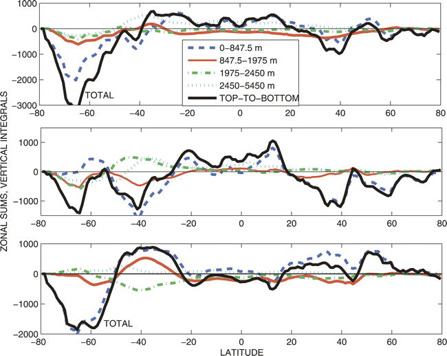
OCEAN STATE ESTIMATION FOR CLIMATE RESEARCH T LEE1 T

Figure 1. Zonal sums of the trends in vertical integrals of the (top) model density anomaly (kg m⁻² yr⁻¹), (middle) from temperature pattern alone, and (bottom) from salinity alone. Solid, black curve is the total top-to-bottom change. Other color curves represent contributions from different depth ranges as shown in the legend. After Wunsch et al. (2007).

Meridional circulation and heat transports:

Meridional Overturning Circulations (MOCs) play an important role in regulating meridional heat transport in the ocean that affects climate variability. Direct measurement or inference of MOCs and meridional heat transport with observations are difficult. Again, ocean reanalyses provide an important tool to characterize and quantify these variables and understand the mechanisms of their variations. For instance, estimates of volume, heat, and freshwater transports of the global ocean have been obtained by fitting an OGCM to WOCE data (Stammer et al. 2003), which facilitates the analysis of interannual to decadal changes of these transports in the ocean (e.g., Köhl and Stammer 2007). Many studies have used various ocean reanalysis products to study regional MOCs and their relations to heat transport and heat content changes. Some examples are described below.

Lee and Fukumori (2003) used an ECCO assimilation product to study the shallow MOC that connects the tropical and subtropical Pacific Ocean, the so-called subtropical cell (STC). The interannual-decadal variability of the lower branches of the STC, the pycnocline flow, is found to exhibit a zonal structure characterized by anti-correlated variability of the western-boundary currents and interior flow. As such, the western-boundary and interior flows play opposite roles in charging and discharging upper-ocean heat content in the tropical Pacific with the interior flow being more dominant. This process has important implication to the understanding of ENSO and its decadal modulation and indicates the need to have sustained in-situ measurements near the western boundary, a region not well resolved by existing observing systems. The partial compensation of boundary and interior flow associated with the Pacific STC has been confirmed by several subsequent studies, for example, by Schott et al. (2007) based on the G-ECCO product (Figure 2). The multi-decadal G-ECCO and SODA products have also been used to study the structure and variability of STCs in the Atlantic, Indian, as well as the Pacific Oceans (e.g., Shoenefeldt and Schott 2006, Schott et al. 2007 and 2008, and Rabe et al. 2008).

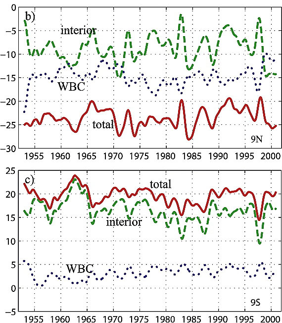
OCEAN STATE ESTIMATION FOR CLIMATE RESEARCH T LEE1 T

Figure 2. Anti-correlated variability of western boundary current (WBC) and interior pycnocline flow at 9°N (upper) and 9°S (lower) in the Pacific, illustrating the opposite roles of WBC and interior flow in charging/discharging tropical Pacific heat content (with the interior flow being more dominant). The results (Schott et al. 2008), based on the G-ECCO product, confirm the finding of Lee and Fukumori (2003) based on a shorter ECCO product.

Ocean reanalyses have also been applied to the studies of MOC away from the tropics. For example, Cabanes et al. (2008) used an ECCO reanalysis product to study the mechanism of interannual variability of MOC in the subtropical and subpolar North Atlantic. They found that the variability of the North Atlantic MOC is correlated with the North Atlantic Oscillation (NAO). In the subtropical North Atlantic, the estimated MOC variability is well correlated with the east-west difference in pycnocline depth, which reflects the zonal pressure gradient that drives the meridional flow associated with the MOC (Figure 3). The variability in the east-west difference of pycnocline depth is primarily associated with fluctuations of the pycnocline depth near the western boundary due to a substantially larger Ekman pumping in the western part of the basin that is correlated with NAO. The identified mechanism would be helpful to the interpretation of dominant interannual variability captured by in-situ monitoring systems for the MOC (e.g., the RAPID array).

Decadal change of the North Atlantic MOC has been a topic of extensive discussion since the analysis by Bryden et al. (2005) using several synoptic hydrographic sections that suggests a substantial slowdown of the North Atlantic MOC at 26°N. Based on estimates by an ECCO-GODAE product, Wunsch and Heimbach (2006) found a much weaker but statistically significant decrease in the strength of the MOC at 26°N as described by the northward volume transport above 1200 m. However, it is accompanied by a strengthening of the deeper meridional circulations, i.e., the southward outflow of North Atlantic Deep Water and northward infow of abyssal water. The decrease of meridional heat transport is not statistically significant. An analysis of ECMWF’s operational ocean reanalysis (Balmaseda et al. 2007) shows that the assimilation significantly improves the time-mean estimates of MOC strength (Figure 3). The resultant estimate of MOC strength at 26°N shows only a weak decreasing trend. No decrease in heat transport is found because the enhanced vertical temperature gradient due to near-surface warming counteracts the decrease in the strength of the MOC. Moreover, the weakening MOC at 26°N is accompanied by an increasing trend in MOC strength at 50°N. The estimates by Balmaseda et al. (2007) are consistent with those of Bryden et al. (2005) for the three points between 1980 and 2000. However, both Wunsch et al. (2006) and Balmaseda et al. (2007) discussed the large high-frequency fluctuations in MOC strength. Such fluctuations could cause aliasing when one attempts to infer low-frequency changes using synoptic hydrographic measurements (Wunsch et al. 2006).

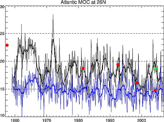
OCEAN STATE ESTIMATION FOR CLIMATE RESEARCH T LEE1 T

Figure 3. Meridional overturning circulation (MOC) variability at 26°N. The time evolution of the MOC for ECMWF’s ocean reanalysis (black) and for the no-assimilation run (blue) is shown using monthly values (thin lines) and annual means (thick lines). Over-plotted are the annual-mean MOC values from Bryden et al. (2005) based on synoptic hydrographic sections and Cunningham et al. (2007) based on RAPID mooring data (green circle). After Balmaseda et al. (2007).

Köhl and Stammer (2008b) also investigated decadal MOC changes as estimated by the G-ECCO 50-year long product. A special focus of their study was is on the maximum MOC values at 25 degree N. Over this period the dynamically self-consistent synthesis stays within the error bars of Bryden et al., but reveals a general increase of the MOC strength. The variability on decadal and longer time scales is decomposed into contributions from different processes. Changes in the model's MOC strength are strongly influenced by the southward communication of density anomalies along the western boundary originating from the subpolar North Atlantic which are related to changes in the Denmar Strait overflow but are only marginally influenced by water mass formation in the Labrador Sea. The influence of density anomalies propagating along the southern edge of the subtropical gyre associated with baroclinically unstable Rossby waves is found to be equally important. Wind driven processes such as local Ekman transport explain a smaller fraction of the variability on those long time scales.

Water mass analyses

Fukumori et al. (2004) used an ECCO product and the adjoint tool to quantify the origin of the NINO3 water in the eastern equatorial Pacific (i.e., the relative contributions of source waters from various parts of the North and South Pacific). They also examined the destination of the NINO3 waters and found that, while NINO3 waters primarily came from the eastern part of the subtropical gyre (the subduction region), the NINO3 waters carried by the surface flow mostly end up in the recirculation region in the western subtropical oceans. Thus, where the NINO3 waters came from and where they are going form an “open circuit” on advective time scales, which is a very different picture from the zonally averaged meridional transport stream function that mis-leadingly depicts a closed loop of meridional circulation. Using the same technique, Wang et al. (2004) investigate the cause for the interannual co-variation of salinity and temperature in the Pacific cold tongue region (higher salinity coinciding with higher temperature during El Nino, vice versa). They found that the anomalous advection of higher salinity waters from the South Pacific (off the equator) was the cause for the salinity variation, which is very different from the mechanism causing interannual variation of cold-tongue temperature (the latter is dominated by interannual change in local upwelling and vertical mixing).

Toyoda et al. (2008) used Japan’s K-7 system product and tool to study the processes responsible for interannual variation of eastern part of the subtropical mode water in the North Pacific and identified three mechanisms (1) salinity convergence by Ekman flow in the preconditioning phase during summer and autumn, (2) solar insolation affected by the amount of stratocumulus in the preconditioning phase, and (3) wintertime surface cooling. They also suggested that the counterpart in the South Pacific exhibited a similar interannual variability and could be explained by the mechanisms described above. Masuda et al. (2006) used the K-7 system and the adjoint method to study source water and processes associated with the inversion layer in the subarctic North Pacific. They found that a deep center of the inversion layer was mostly associated with source waters from the Kuroshio region whereas a shallower center of the inversion layer involved source water from the Gulf of Alaska.

Mixed-layer heat budget analyses

Some of the ocean reanalysis products (e.g., the ECCO family products and Japan’s K-7 product) are characterized by their physical consistency such that the estimated oceanic state and surface forcing satisfy the governing equations of the underlying models. Therefore, they allow the closure of property budgets, which greatly facilitates such analysis as heat balance. For example, Kim et al. (2004 and 2007) and Halkides and Lee (2008) used ECCO products to study seasonal-to-interannual heat balance of the mixed layer in subtropical North Pacific, equatorial Pacific, and tropical Indian Ocean.

Kim et al. (2007) shows that advective processes that control the interannual anomaly of NINO3 temperature as a whole are dominated by large-scale processes, namely, the variations in zonal advection of warm-pool water into the cold-tongue region, meridional advection by Ekman flow, and vertical advection by upwelling. The picture is very different from local balance of mixed-layer temperature at individual locations of TOGA-TAO moorings. The latter is significantly affected by smaller-scale currents associated with tropical instability waves that primarily redistribute heat within the NINO3 region rather than causing heat exchange across the NINO3 boundaries. The analysis of local balance of mixed-layer temperature in the eastern tropical Indian Ocean (Halkides et al. 2008) shows that the advection of heat in the region has substantial spatial variations such that the spatial average of heat advection is not statistically significant. The region is found to be characterized by three dynamically different circulation regimes that are associated with heat advection by the Wyrtki Jet in the equatorial zone, upwelling off the Java-Sumatra coasts, and the South Equatorial Current further south. Spatial average of local heat advection obscures these important differences in regional dynamics and thermodynamics. Physically consistent ocean reanalyses make such studies possible and improve the understanding local versus large-scale heat balance. The results help interpret local heat budget analysis based on sparse in-situ measurements such as mooring observations.

2.2 Intercomparison

As part of the ongoing CLIVAR/GODAE global ocean reanalysis evaluation effort, many ocean reanalysis projects have participated in an intercomparison that involves many diagnostics quantities, including the comparison among reanalysis products and comparison with observations. The objectives of such intercomparison are to (1) examine the consistency of the reanalyses (though multi-product comparison), (2) evaluate the accuracy of these products (by comparison with observations), (3) provide some level of uncertainty estimate for a given diagnostics based on the spread of the ensemble, (4) identify areas where ocean reanalyses need improvement, and (5) define the requirement of observational accuracy needed to distinguish the quality of the reanalyses and identify future observational need. The following is an example of such intercomparison and the relations to the objectives described above.

Figure 4 shows a comparison of the seasonal and non-seasonal anomalies of the volume transport of the Indonesian throughflow (ITF), defined as the top-to-bottom volume transport integrated across and summed over the Lombok and Ombai Straits and Timor passages. These products are contributed by the assimilation groups: ECCO, GFDL, and SODA from the US, CERFACS and MERCATOR from France, G-ECCO from Germany, MOVE-G and K-7 from Japan, and INGV from Italy. The products are generally consistent in terms of stronger (weaker) ITF transport during boreal summer (winter) (Figure 4a) and during La Nina (El Nino) (Figure 4b). Note that a negative anomaly of ITF transport indicates a stronger ITF because the time-mean ITF is negative (southward).

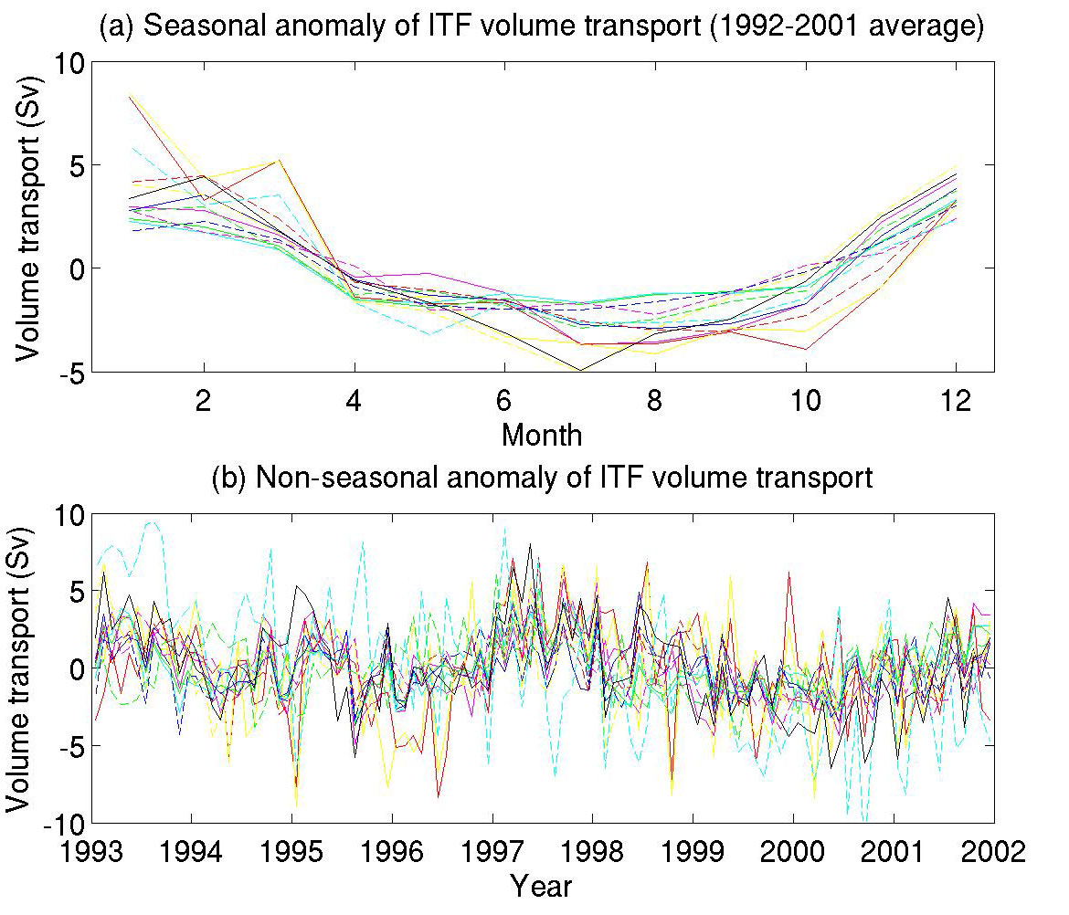
OCEAN STATE ESTIMATION FOR CLIMATE RESEARCH T LEE1 T

Figure 4. Comparison of (a) seasonal anomaly (composite over the years of 1993-2001) and (b) non-seasonal anomaly (with the respective 1993-2001 seasonal cycle removed) for 13 ocean reanalysis products.

The averaged r.m.s. difference among the products is 2.3 Sv for total anomaly (without time mean). The r.m.s. difference for the seasonal, non-seasonal, and interannual (annually averaged non-seasonal) anomalies among the products are 1, 2, and 1 Sv, respectively. The averaged magnitude of variability for these products is 3.6 Sv. This is larger than the 2.3-Sv r.m.s. difference among the products, indicating that the physical signal in the products is larger than the noise. The averaged time-mean ITF volume transport is 13.8 Sv, which is consistent with the averaged inference from observations to within observational uncertainty. However, the r.m.s. difference among the time-mean estimates, 3.7 Sv, is substantially larger than that for the variability mentioned above. In other words, the consistency for the time mean is not as good as that for the variability. What are the implications of the results of the intercomparison? They highlight the need to further understand the factors that control the time-mean ITF transport in models (e.g., topography, mixing, time-mean forcing, the lack of data constraint over the period of study). Moreover, the averaged r.m.s. difference among different products described above provide a minimal requirement for observational accuracy because that is what is needed to distinguish the quality of these ocean reanalyses and to constrain them effectively.

2.3 Signal and uncertainty in ocean reanalyzes

As described earlier, one purpose of the intercomparison is to estimate the uncertainty of an estimated quantity from different reanalysis products. Estimating uncertainty is a major challenge. In addition to the three dimensional estimation of the ocean state at a given time (analysis problem), the estimation of the time evolution is also required in a reanalysis. The time evolution represented by an ocean reanalysis will be sensitive to the time variations of the observing system, to the errors of the ocean model, atmospheric fluxes and assimilation system, which are often flow dependent, and not easy to estimate. In cases where the complexity is too large to be tackled analytically, the ensemble methods can offer a helping hand. So, in the same way as the ensemble of multi-model forecasts is used to get an estimation of the uncertainty of future climate projections, and ensemble of different reanalysis products can be used to get a first glance of the time evolution and uncertainty of the climate reconstructions, although the caveats of the ensemble methodology should be taken into account when interpreting the results.

This approach was followed by Balmaseda and Weaver 2006 in the comparison of ocean reanalysis organized by the CLIVAR GSOP (http://www.clivar.org/organization/gsop/synthesis/synthesis.php). The results from 20 global ocean reanalysis products, with different models, assimilation methods and forcing fluxes, were gathered together to examine the time evolution of the upper ocean temperature and salinity. One of the reanalysis did not include any ocean model. Some of them did not include any ocean observations, being the result of ocean models forced by atmospheric forcing fluxes. For the early years (1960-1980) there were only seven available products. For the period 1993-2002 there were 20 products, and very few were available for post-2002. The scarcity of reanalyses products for the last few years hampers the assessment of uncertainty on recent climate signals.

Figure 5 shows the signal-to-noise ratio of the interannual variability of temperature (left) and salinity (right) in the upper 300m (T300 and S300 in what follows) for different regions. The signal is estimated as the temporal standard deviation of the ensemble mean, and the noise as the ensemble spread. For the period 1960-2002, the North Atlantic (NATL, 30N-60N) stands out as the region where the temperature signal dominates the noise. The signal is also quite clear in Equatorial Pacific (EQPAC, 5S-5N), the Tropical Atlantic (TRATL ,20S-20N) and the GLOBAL ocean. In the most recent period (1993-2002), the signal to noise ratio in temperature is larger than 1 in most areas, and the Equatorial Pacific clearly stands out. In contrast, the upper ocean salinity signal to noise ratio is less than one almost everywhere, except for the Equatorial Pacific, where it is close to 1.

The climate signals and source of uncertainty can be investigated further. Figure 6 shows the time evolution of T300 in four regions: GLOBAL ocean, North Atlantic, North Pacific (30-60N) and Equatorial Pacific. The grey shade shows the spread among the 20 different ocean reanalyses. They have been grouped according to their forcing fluxes and use of data. The red shade shows the results for only those reanalysis that use ER40 forcing fluxes (Uppala et al 2005). These have been further subdivided into reanalysis without data assimilation (blue) and with data assimilation (green). The inset in each figure shows the size of the average spread for each of these groups. The difference between grey and red can be taken as a measure of uncertainty due to forcing fluxes. The size of the blue spread is representative of uncertainty due to using different ocean models. The size of the green spread is due to the differences in model an assimilation method. The difference between green and blue is indicative of the ability for the data assimilation to reduce (or on the contrary to increase) the uncertainty of the climate signals. Results indicate that the uncertainty induced by the forcing fluxes is comparable to the uncertainty due to ocean model formulation. In the regions shown here, the assimilation of ocean data reduces the spread of the model-only runs, especially noticeable in the Equatorial Pacific. However, the assimilation can increase the uncertainty in the temperature field in the tropical Atlantic and Indian Ocean and in the salinity field almost everywhere (not shown). The fact that the assimilation can increase the uncertainty points towards the need for more robust assimilation methods that better handle model and data errors and the need for additional observations.

In spite of the large uncertainty, results shown in Figure 6 indicate that there are clear climate signals. For instance, the increasing trend in the global upper ocean heat content is visible, as well as decadal variability: lower values in the 60’s, a maxima during at the beginning of the 80’s, another drop in the mid 90’s and an increasing trend ever since. The magnitude of the decadal signals is stronger with assimilation than with the free ocean model. Whether the intensification of the decadal signal is due to the XBT’s bias (e.g., Gouretski and Koltermann 2007) or to other reasons (for instance, to the lack of information in the forcing fluxes) need to be investigated farther. The decadal signals and increasing trend is also visible in the North Atlantic, which shows the largest acceleration in the warming in the late 90’s. After 2000 however warming seems to stabilize, or even decrease. Unfortunately the uncertainty increases tremendously in the last few years. The North Pacific variability is more dominated by decadal variability rather than by secular trends. There is quite a pronounced rapid warming in the late 80’s, which may be related to the changes in the gyre circulation reported by Suga et al 2002, Taneda et al 2000. The origins of this shift and its role in the global climate need further investigation. The Equatorial Pacific is the region where the interannual variability is quite clear, and where the uncertainty has been decreasing steadily with time, probably due to the enhancement of the TOGA-TAO system. The interannual variability in the Equatorial Pacific upper ocean heat content shows a clear downward trend, as has been described by Balmaseda et al (2008). The relation of this trend in heat content with the the weakening of the Walker Circulation (Vecchi et al 2006, Scott and Smith 2007) needs further investigation.

OCEAN STATE ESTIMATION FOR CLIMATE RESEARCH T LEE1 T

Figure 5. Signal to noise ratio for the time evolution of temperature and salinity in the upper 300m (T300 and S300) in different regions. The estimates have been done separately for the period 1960-2002 and for the most recent period 1993-2002.

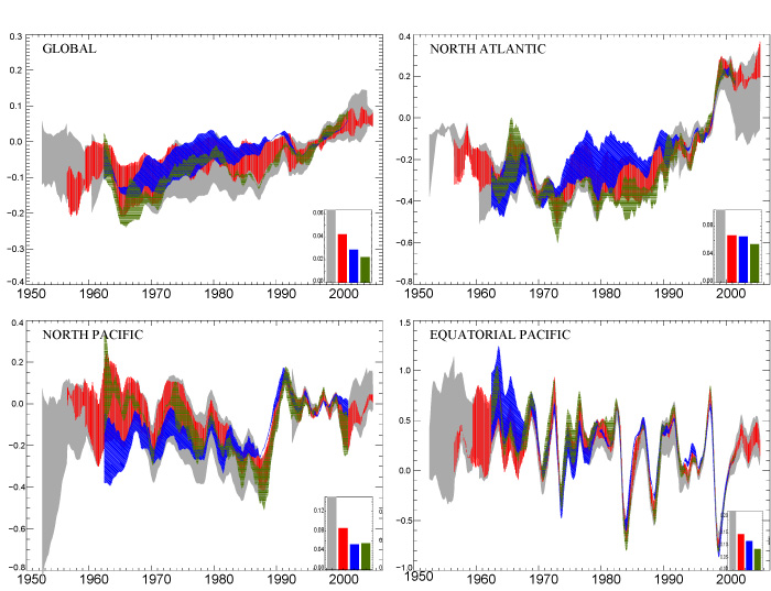
OCEAN STATE ESTIMATION FOR CLIMATE RESEARCH T LEE1 T

Figure 6. Time evolution and spread of the upper 300m average temperature in different regions. The spread resulting from using 20 different ocean reanalysis is shown in grey. Those reanalysis that use the same forcing fluxes (ERA40) are shown in red. The difference between grey and red is indicative of uncertainty arising from the forcing fluxes. The blue shading is indicative of the uncertainty arising from the ocean model formulation, since it groups ocean simulations which do not assimilate data and differ only on the ocean model. The same models, but this time using data assimilation, are shown in green. The difference between blue and green is representative of the effect of the assimilation on the signal and on the spread.

3. Summary and Challenges ahead

As part of CLIVAR’s and GODAE’s effort in the past decade, significant advancement has been achieved in ocean state estimation efforts that are geared towards climate research. A suite of global ocean reanalysis products have been produced and updated on a routine basis. There have been an ever increasing number of applications of these products for oceanographic and climate-related studies over a wide range of topics. The existence of these products also allows a comprehensive intercomparison to evaluate the consistency and fidelity of the various climate-related diagnostic quantities estimated from different products. The intercomparison help identify areas that need improvement in ocean reanalysis and observing systems. Despite the significant advancement in ocean reanalyses, many challenges lay ahead. The ocean data assimilation groups need to work closely with the modeling community to improve the model physics, especially those associated with the bias of the mean state.

The estimates of data and model errors dictate the outcome of the state estimation for a given model. Therefore, the ocean reanalysis community needs to work closely with the observational community in obtaining robust estimates of data errors, an important issue that is often dealt with only by the assimilation groups. The uncertainty in the observations associated with such factors as changing fall rate of XBTs over the past few decades and some biased ARGO data in the past few years are among examples that more effort is needed to estimate data error. Moreover, much research is still required to understand model errors. In particular, we need to identify the sources of model errors and determine if appropriate new control variables can be adopted to account for such error sources (e.g., internal model errors associated with mixing parameterizations).

Computational resources remain to be a critical issue for estimation effort based on the ensemble and adjoint methods because it limits the ensemble size and model resolution that one can afford. Finally, the coupled nature of the climate system prompts for a coupled approach for state estimation that includes components of the climate system (such as the atmosphere, cryosphere, hydrosphere, and biogeochemistry) in order to properly account for the potential feedback among different elements of the climate systems. Currently, coupled ocean-atmosphere, ocean-ice, and ocean physics-biochemistry data assimilations are still in their infancy and are expected to pick up momentum in the coming decade.

References

Balmaseda, M.A. , D. Anderson and F. Molteni (2008). Climate variability from the new ECMWF Ocean Reanalysis System ORA-S3. Third WCRP Conference on Reanalysis. http://wcrp.ipsl.jussieu.fr/Workshops/Reanalysis2008/Documents/G2-264_ea.pdf

Balmaseda, M.A., G.C. Smith, K. Haines, et al. 2007: Historical reconstruction of the Atlantic Meridional Overturning Circulation from the ECMWF operational ocean reanalysis. Geophys. Res. Lett., 34, L23615, doi:10.1029/2007GL031645.

Cabanes, C., T. Lee, and L.-L. Fu, 2008: Mechanisms of Interannual Variations of the Meridional Overturning Circulation of the North Atlantic Ocean. J. Phys. Oceanogr., 38, 467-480.

Carton, J.A., B.S. Giese, 2008: A reanalysis of ocean climate using Simple Ocean Data Assimilation (SODA). Mon. Wea. Rev., 136, 2999-3017.

Domingues, C.M., J.A. Church, N.J. White, et al. Improved estimates of upper-ocean warming and multi-decadal sea-level rise. Nature. 453, 1090-U6.

Fukumori, I., T. Lee, B. Cheng, and D. Menemenlis, 2004: The origin, pathway, and destination of NINO3 water estimated by a simulated passive tracer and its adjoint. J. Phys. Oceanogr., 34, 582-604.

Gouretski V., K. P. Koltermann (2007), How much is the ocean really warming?,Geophys. Res. Lett., 34, L01610, doi:10.1029/2006GL027834.

Halkides, D., and T. Lee, 2008: Mechanisms controlling seasonal-to-interannual mixed-layer temperature variability in the southeastern tropical Indian Ocean. J. Geophys. Res., submitted.

Kim, S.-B., T. Lee, I. Fukumori, 2007: Mechanisms controlling the interannual variation of mixed layer temperature averaged over the NINO3 region. J. Clim., 20, 3822-3843.

Kim, S.-B., T. Lee, and I. Fukumori, 2004: The 1997-99 abrupt change of the upper ocean temperature in the northcentral Pacific. Geophys. Res. Lett., 31, L22304, doi:10.1029/2004GL021142.

Köhl, A., and D. Stammer, 2008a: Decadal sea level changes in the 50-year GECCO ocean synthesis. J. Clim., 21, 1866-1890.

Köhl, A., D. Stammer, and B. Cornulle, 2007: Interannual to decadal changes in the ECCO global synthesis. J. Phys. Oceanogr., 37, 313-337.

Köhl, A. and D. Stammer, 2008b: Variability of the meridional overturning in the North Atlantic from the 50-year GECCO state estimation. J. Phys. Oceanogr., 38, 1913 -1930.

Lee, T., and I. Fukumori, 2003: Interannual to decadal variation of tropical-subtropical exchange in the Pacific Ocean: boundary versus interior pycnocline transports. J. Climate. 16, 4022-4042.

Masuda, S., T. Awaji, N. Sugiura, T. Toyoda, Y. Ishikawa, K. Horiuchi (2006), Interannual variability of temperature inversions in the subarctic North Pacific, Geophys. Res. Lett., 33, doi:10.1029/2006GL027865.

Masuda, S., T. Awaji, T. Toyoda, Y. Shikama, Y. Ishikawa (2008), Temporal evolution of the equatorial thermocline associated with the 1991-2006ENSO: A possible cause of ENSO irregularity, J. Geophys. Res. (submitted).

Power, S. B., and I. N. Smith (2007), Weakening of the Walker Circulation and apparent dominance of El Niño both reach record levels, but has ENSO really changed?, Geophys. Res. Lett., 34, L18702, doi:10.1029/2007GL030854.

Rabe, B., F.A. Schott, and A. Köhl, 2008: Mean circulation and variability of the tropical Atlantic during 1952-2001 in the GECCO assimilation fields. J. Phy. Oceanpgr., 38, 177-192.

Schoenefeldt, R., and F. A. Schott, 2006: Decadal variability of the Indian Ocean cross-equatorial exchange in SODA. Geophys. Res. Lett., 33, L08602, doi:10.1029/2006GL025891.

Schott, F.A., L. Stramma, W. Wang , et al., 2008: Pacific Subtropical Cell variability in the SODA 2.0.2/3 assimilation. Geophys. Res. Lett., 35, L10607, doi:10.1029/2008GL033757.

Schott, F.A., W.-Q. Wang, and D. Stammer, 2007: Variability of Pacific subtropical cells in the 50-year ECCO assimilation. Geophys. Res. Lett., 34, L05604, doi:10.1029/2006GL028478.

Stammer, D., C. Wunsch, and R. Giering, et al. 2003: Volume, heat, and freshwater transports of the global ocean circulation 1993-2000, estimated from a general circulation model constrained by World Ocean Circulation Experiment (WOCE) data/ J. Geophys. Res.-Oceans, 108,

Suga, T; Kato, A; Hanawa, K. 2000. North Pacific Tropical Water: its climatology and temporal changes associated with the climate regime shift in the 1970s. Progress in Oceanograph, 47 (2-4): 223-256.

Toyoda, T., T. Awaji, S. Masuda, N. Sugiura, H. Igarashi, T. Mochizuki, and Y. Ishikawa: Interannual variability of North Pacific eastern subtropical mode water formation in the 1990s derived from a 4-dimensional variational ocean data assimilation experiment. (submitted to J. Geophys. Res.)

Wang, O., I. Fukumori, T. Lee, and B. Cheng, 2004: On the cause of eastern equatorial Pacific Ocean T-S variations associated with El Nino. Geophys. Res. Lett., 31, L15310, doi:10.1029/2004GL02472.

Wunsch, C., R.M. Ponte, P. Heimbach, 2007: Decadal trends in sea level patterns: 1993-2004. J. Clim., 20, 5889-5911.

Wunsch, C. and P. Heimbach, 2007: Estimated decadal changes in the North Atlantic meridional overturning circulation and heat flux 1993-2004. J. Phys. Oceanogr., 36, 11, 2012-2024.

2019年第三季度本校论文SCI收录情况检索数据库：WEB OF SCIENCE 核心合集检索年代：2019年迄今检索策略：机构扩展：GUANGDONG OCEAN UNIVERSITY
2ND PACIFIC OCEAN REMOTE SENSING CAPACITY BUILDING WORKSHOP ON
A DROP IN THE OCEAN? – CZECHOSLOVAK TROOPS IN

Tags: climate research, the climate, climate, state, ocean, estimation, research