ANIMATION OF POWER ELECTRONICS AND ELECTRICAL DRIVES PETER J
11ème Animation Karting af 2015 – ClotANIMATION MARKETING MESSAGES JANUARY 2020 ANIMATION MARKETING
1884 IBM IMS SCENARIO ANIMATION PART 1 SCRIPT –
ACCUEIL EN SERVICE DE RÉANIMATION ACCUEIL EN RÉA
ANIMATION ACTIVITÉ PHYSIQUE ET HANDICAPS – ATELIER DANSE DÉROULEMENT
ANIMATION AND EPISTEMOLOGY IVY KIDRON DIEUDONNE (1992) WROTE
Animation of Power Converters and Electrical Drives
Animation of Power Electronics and Electrical Drives.
Peter J. van Duijsen
Simulation Research
P. O. Box 397, NL-2400 AJ,
Alphen aan den Rijn, The Netherlands
Tel: +31 172 492353, Fax: +31 172 492477
Email: [email protected]
Dan Lascu
Politehnica University Timişoara
Faculty of Electronics and Telecommunications,
Bd. Vasile Pârvan 2, 1900 Timişoara, Romania
Phone: 0040-56-204332, ext. 642, Fax: 0040-56-190608,
Email: [email protected]
Abstract
In this paper a new multilevel simulation/animation tool Caspoc®, [Simulation Research, 2001] is described, which during simulation animates the power electronic circuit. The user sees the level of the node-voltages, the level of the branch currents and most important, he can see the current path in the circuit. The simulation tool can animate any power electronic circuit or electrical drive.
Examples of power electronic and electrical drive animations are given, which show the advantage of animation.
Keywords
Animation, modeling, simulation, power electronics, electrical drives, teaching
1.Introduction
Teaching and understanding Power Electronics and Electrical Drives have been done with the use of books and the blackboard. Many of us will remember the times drawing the basic waveforms of converter operation on paper while keeping the state of the converter in mind.
Simulation made a change here, because it gave us the possibility to use a computer for drawing while keeping our attention to the operation of the converter. Simulation enabled us to study the behavior for different parameters and conditions. Still the user has to keep the converter in mind and he has to make an interpretation of the simulation results.
The next logical step is to present the operation of the converter as a result of the simulation. Accustomed as we are to cartoons, this logical step is called animation. During the simulation the converter operation is presented as a cartoon. The resulting animation gives the user an insight in the converter operation, which was not possible with books and blackboard. Even a real operating converter does not show so many operating details as during animation, simply, because of the high switching frequencies. For example, even in a 50Hz rectifier, the step by step operation goes too fast to follow by the human brain and we use a scope to store the waveforms during the operation.
In animation you can actually see the converter switching, see how integrators in controllers build up charge and how motors start to rotate.
In section 2, an introduction is given in the mathematical methods, which are used in simulation programs for Power Electronics and Electrical Drives. The importance of simulation for education is briefly described in section 3. A short discussion on modeling of components is presented in section 4. In section 5 the visualization of simulation results is discussed. The fact that animation is not just a toy is described in section 6 and the impact of the animation on the simulation speed is discussed in section 7. The examples in this paper will focus on the animation of power electronic circuits and electrical drives. The user has the possibility to define his own motion control models in a high-level programming or a block-diagram, enabling him to model, for example, a field oriented controller or controls for application specific drives, such as fans, pumps and automotive applications. Various examples of animation, for example the Vienna-Rectifier, conclude this paper in section 8 to 13, with final concluding remarks in section 14.
2.Modeling and Simulation methods
Simulation starts to become an accepted tool for the design of power electronics and electrical drives. Over the last 30 years there have been remarkable advances in tools for the simulation of power electronics and electrical drives. Not only advances in the user interface of the programs, but also advances in the underlying methods on which these simulation tools are based.
For power electronics and motion control industries, various modeling and simulation packages are available. The integration of modeling and simulation for both motion control and power electronics into one package is not so wide spread.
For the modeling of electric circuits and dynamic systems, there are generally three methods.
The State-Space approach, [Schwarz, 1987] is used in Block-diagram oriented programs, such as Simulink. The advantages of the state-space model are simplicity and simulation speed. The disadvantage is the difficulty to derive the state space equations from a circuit.
The Modified Nodal Analysis (MNA) method, [Ho, 1975], is used in Spice-based programs. The advantage is the easy mathematical model generation from a circuit. The disadvantages are the convergence problems caused by semiconductor models.

Figure 1 : Complexity of models.
The modeling of a component in a Power Conversion System (PCS) is not unique. Depending on the need of the user, a model can be either simple, detailed, or can contain just enough details to model the time-domain behavior satisfactory.
The complexity of the mathematical model is not necessarily related to the complexity of the model of the component. As shown in figure 1, a simple model can contain a (non-linear) acausal mathematical relation and therefore a Differential Algebraic Equation DAE, [Schwarz, 1987], has to be used for the mathematical model:
![]() (1)
(1)
The
DAE describes the non-linear, possible acausal, relations among the
time-varying state
variables x(t),
their time-derivative
![]() (t),
the variables
y(t)
and the input
variables
u(t)
of a PCS.
(t),
the variables
y(t)
and the input
variables
u(t)
of a PCS.
On the other side, if a more detailed model doesn't contain any acausal relations, it can be described by a Ordinary Differential Equation ODE:
 (2)
(2)
Equation (2) is used in Block-diagram programs such as Simulink.
The SPICE® program is based on the MNA method. Suppose a model can be formulated as:
![]() (3)
(3)
The parameters of the matrix A are dependent on the variables and state variables in the vector x(t). Vector b(t) stores the values of the independent sources. The time derivative of x(t) is replaced by a numerical integration approximation, where the parameter h is the step size of the numerical integration
Multilevel modeling [Franz, 1990], [Duijsen, 1994] is a technique where different mathematical model descriptions, such as DAE, MNA and ODE, can be combined. A multilevel simulation is based on the total mathematical model of the multilevel model. A multilevel model can contain different types of models. The multilevel modeling technique is advantageous compared to other modeling techniques for two major reasons.
Efficient modeling, because each part of the implementation like the power electronic circuit, the load or the control is described by its most efficient modeling technique. This allows a straightforward description without, for example, modeling an inverter in a block diagram or modeling a control algorithm by lumped circuit elements.
The simulation time can be decreased, because each part of the implementation can be solved more efficiently.
3.Modeling and simulation for education
Modeling and simulation is a valuable tool in the area of education and training. Especially in the field of power electronics and drives, simulation is a more save method to teach. Faults and mistakes made during a simulation cause no damages or risks. To be more precisely, you can learn much more when you can simulate critical events, which are impossible to perform in reality. Take for example the maximum current through an expensive GTO. Destroying a GTO in a simulation is harmless compared to a real destruction of a GTO. Performing only simulations implies no hazardous damages to the surrounding, no replacements, no soldering, no stock of expensive GTOs.
Important for education is the availability of a library with examples. Nearly all large vendors provide examples for their simulation tools. For Spice® and Simulink® tutorials and libraries with examples for power electronics and drives can bought from third-party vendors. For Caspoc® a tutorial especially with power electronics and drive examples is available.
Simulation speed is even for education an important factor. However simulation examples can be structured such that a short simulation time is achieved by either simplifying the example or generalized modeling. Simulation speeds achieved with Spice® and Simulink® are satisfactory, with Caspoc® shorter simulation times can be achieved because of the multilevel modeling. Also of importance is the convergence of the simulation. Here Spice® has a bad performance, which can lead to a struggle with the model. In many cases the effort to make a Spice® simulation, goes mainly to including tricks in the model to enhance convergence. This leads to a waste of time for education, because students should learn how to build models, not to prevent convergence failures. Simulink® and Caspoc® have no convergence problems as known with Spice®.
4.Models
For the simulation of Power Electronics basic models are required, which do not exist in standard simulation programs, such as the early Spice-based programs. Recent Spice-based simulation programs have a library of sub-circuits for Power Electronic components such as the SCR, GTO, Mosfet, IGBT and, for example, electrical machines.
The complexity of the model is a very important aspect in modeling. For most simulations a basic switching behavior is satisfactory. For example, the basic switching behavior of a diode, SCR or GTO, is in many cases satisfactory to model a three-phase rectifier. A linear inductance modeled at the input is enough to simulate the commutation between the diodes in a rectifier. The produced harmonics are basically only depending on the line impedance of the input of the rectifier.
For calculating the efficiency of a SMPS, also the energy that is required to control the Mosfet is important. Here the non-linear gate capacitance has a large influence on the efficiency of the SMPS. In this case a model where the gate charge of a Mosfet is modeled is required. Multilevel modeling simplifies the modeling process for these various components.
5.Visualizing simulation results.
The early simulation programs produced a long list with numerical results. Nowadays most simulation programs offer the presentation of simulation results in graphical windows. The user has the ability to examine these graphical results by using a mouse, to obtain the numerical value at each point in time.
The next step is the visualization of the simulation. Most important in power electronics is the current-path. For example, freewheeling of diodes becomes clear, when the user sees the current-path changing from switches to freewheeling diodes.
The following visualization guidelines are used:
The intensity of the voltage, current or signal is given by the color, which varies from black to red, as defined by a rainbow of colors.
The color of a node in the electric circuit is dependent on the voltage level of that node.
The color of an electric circuit component is dependent on the level of the current through that component.
The color of an electric circuit wire is dependent on the level of the current through that wire.
The color of a wire in the block-diagram is dependent on the level of the signal on that wire.
Certain components animate depending on an event, taking place in the component, such as opening or closing of switches.
6.Importance of animation.
Animation of electric circuit may look like a toy. This is however absolutely wrong. Animation is a viable tool for teaching, gaining insight, checking the behavior, or searching for failure modes.
The advantages for teaching are clear. Students, for example, can see the current-paths in rectifiers or understand the freewheeling and discontinuous mode in SMPS.
For complex topologies, such as the Vienna-Rectifier [Kolar, 1994], animation can be very helpful to understand and verify the principle of the converter. During animation, it becomes clear to the user how the converter is behaving.
During animation, failure modes are detected. Even those failure modes, the user was not aware of. During failure analysis without animation it requires a lot of time to check each component. With animation, each failure is directly displayed, for example a switch is opened or closed at a wrong interval. Or some voltage levels are too high.
7.Practical implementation.
Animation costs time. A simulation should be as fast as possible. Animation slows down the simulation. Therefore the user should have the ability to turn the animation on or off.
If a circuit is animated, the simulation in most cases has to be slowed down, in order to follow the behavior of the system. Therefore the time-consumption of animation is in many cases not a problem.
In order to speed up the animation it is not always necessary to show each simulation step. For example, if a small time step is required for the simulation but the animation is slow varying, compared to the time step, not each time step has to be displayed. This can be achieved by not displaying each time step in the animation. Figure 2 shows a typical dialog box for animation properties.
To visualize the values of voltage and current, two different levels are required. For example a SMPS operating at the AC-mains can have current levels of only up to 1 Ampere. Also the control signals can vary in value from the voltage and current level. Typical control signals can range between 0 and 1, where the on-status of a control signal is clearly signaled by a red color and the off-status is signaled by a black color.

Figure 2: Animation properties.
To prevent that the schematic starts blinking like a Christmas tree, the user should have the possibility to turn on or off various animation effects. For example, the constant display of numerical values at each node can make the schematic very crowded and therefore the user should have the possibility to turn it off.
8.Example Vienna-Rectifier
In figure 3 the Vienna-Rectifier [Kolar, 1994] is displayed. The current-path, which is colored during the animation, is shown thick in this figure. One can see clearly that the complexity of the current-path gives valuable information on the functioning of the converter.
Figure 3: Current-path in the Vienna-Rectifier.
9.Example Buck converter
In figure 4 the animation of a buck converter is shown. In the figure the freewheeling of the diode is shown. The level of the output voltage and the level of the current through the inductance L1 is displayed by two analog meters, which during the animation show the actual value.
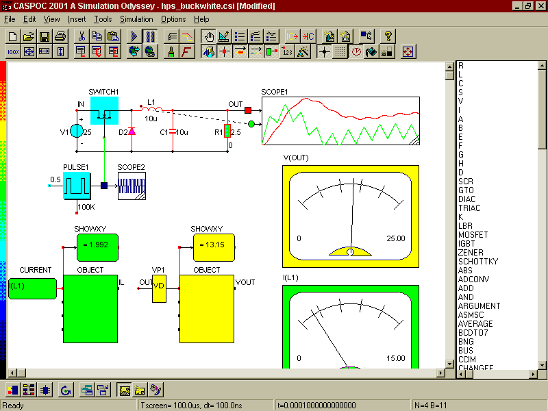
Figure 4: Buck converter with analog meters.
10.Example DC shunt machine with crane
In figure 5 the animation of a DC shunt machine with crane is shown. The DC shunt machine is controlled by a controlled voltage source, which is regulated by a library-block 'Crane Control'. Also a controlled rectifier could have been used here. The library-block modeling the crane includes an object-block, which models the visualization of the crane. Depending on the angle of the axis of the DC shunt machine, the load is lifted by the crane.
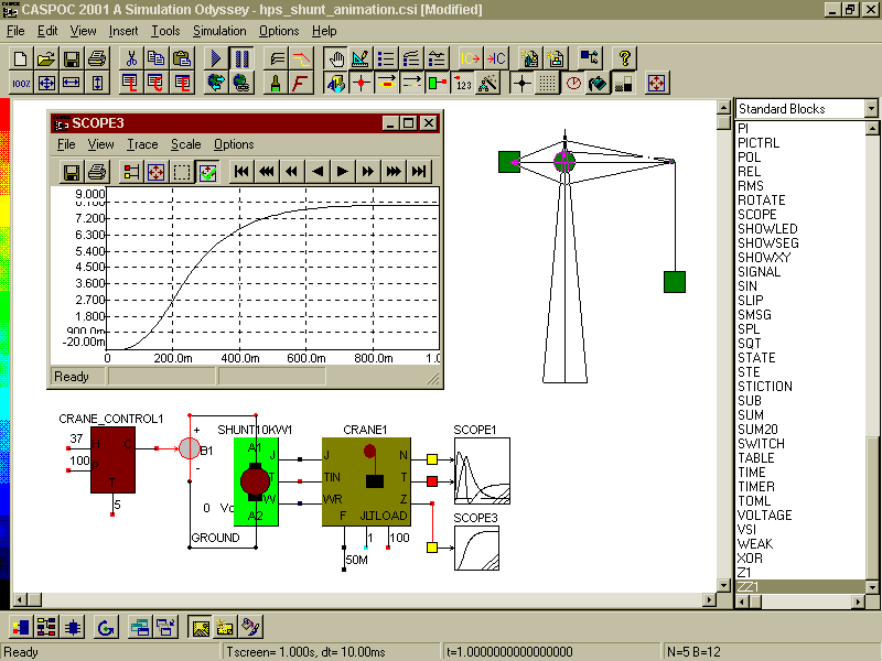
Figure 5: DC shunt machine with crane.
11.Example Switched Reluctance Machine
The model for the Switched Reluctance Machine (SRM) contains a non-linear inductance, which is depending on the position of the rotor and the saturation in the stator. The non-linear inductance is modeled per phase by a function or via a 2-dimensional table.
Figure 6: Switched Reluctance Machine with current control.
In figure 6 the model for a SRM is shown. The SRM is modeled inside the library block SRM46, which contains the model for a 6-stator and 4-rotor pole machine. On the left side the electrical connection to the converter is made. The inductances of the machine are connected to the converter via the nodes L1A-L1B, L2A-L2B and L3A-L3B. The parameters for the machine are supplied via a .model database as shown below:
.model srm68_1 user br=0.436 bs=0.349 jr=0 lmax=110m lmin=10m nr=6 ns=8 r=50
.model srm68_2 user br=0.436 bs=0.349 jr=0 lmax=210m lmin=10m nr=6 ns=8 r=20
.model srm64 user br=0.581 bs=0.465 jr=0 lmax=2.84m lmin=0.284m nr=4 NS=6 r=0.8
The name of the .model has to be specified in the block MName. The parameters for the machine are supplied at the bottom of the model.
On the right side a mechanical load is connected to the SRM. The load has an inertia of 54Kg.m2 and the torque Tload from the load equals 13.5*N, where N is the number of revolutions per min. In the scope at the right side of the Load block the speed of the rotor is displayed.
At the top side of the SRM the control signals and the currents through the inductances are exported. With a current regulator the current through each inductance is limited between 870 and 890 Ampere, using two comparators, a Flip-Flop and an AND-gate. The IGBT's are only closed if the position of a rotor pole is in front of a stator pole and is indicated by the nodes C1, C2 and C3.
During the animation the rotor is rotating and the
value of L1 is displayed in a scope. The dependence of the inductance
on the position of the rotor is visualized during the animation.
12.Example stepper motor with half step control
In figure 7 a bipolair stepper motor with half step control is displayed. The current through the inductances La and Lb is measured and in the block STBERBIP, the torque produced by the machine is calculated. On the right side of the machine, a Load block is connected modeling a linear mechanical load. The rotor speed and the produced torque are displayed in scope 2. The torque pulses are clearly visible.
Depending on the position and speed of the rotor, the back-emf (EA and EB) is calculated in the block STBERBIP and is modeled in series with the inductances LA and LB, where also the resistance (R=100Ohm) is modeled.
The position of the rotor is exported on the node H1 at the top of the block for the stepper motor. This node is connected to the block Object where using the parameter p1 the animation object for the stepper motor is defined. Depending on the value of H1, which varies from 0 to 2*π, the rotor is rotating during the animation.
Figure 7: Stepper motor with half step control.
The block STUNIHALF, which produces a fixed pulse pattern for the Mosfet's, regulates the stepper motor. As can be seen in the animation, the currents through La and LB in figure 7 are positive and therefore the rotor is positioned as shown in figure 7. In figure 7 the Mosfet's where the gates GA1 and GB1 are positive are conducting. The position of the fixed pulse pattern is given by the value of A which is varying from 0 to 2*π.
13.Example brushless DC machine with 6-pulse control
In figure 8 the Brushless DC machine with 6-pulse control and IGBT inverter is displayed. The block BLDCM models the brushless machine, where on the left side the block is connected to the inverter and on the right side, the mechanical load is connected.
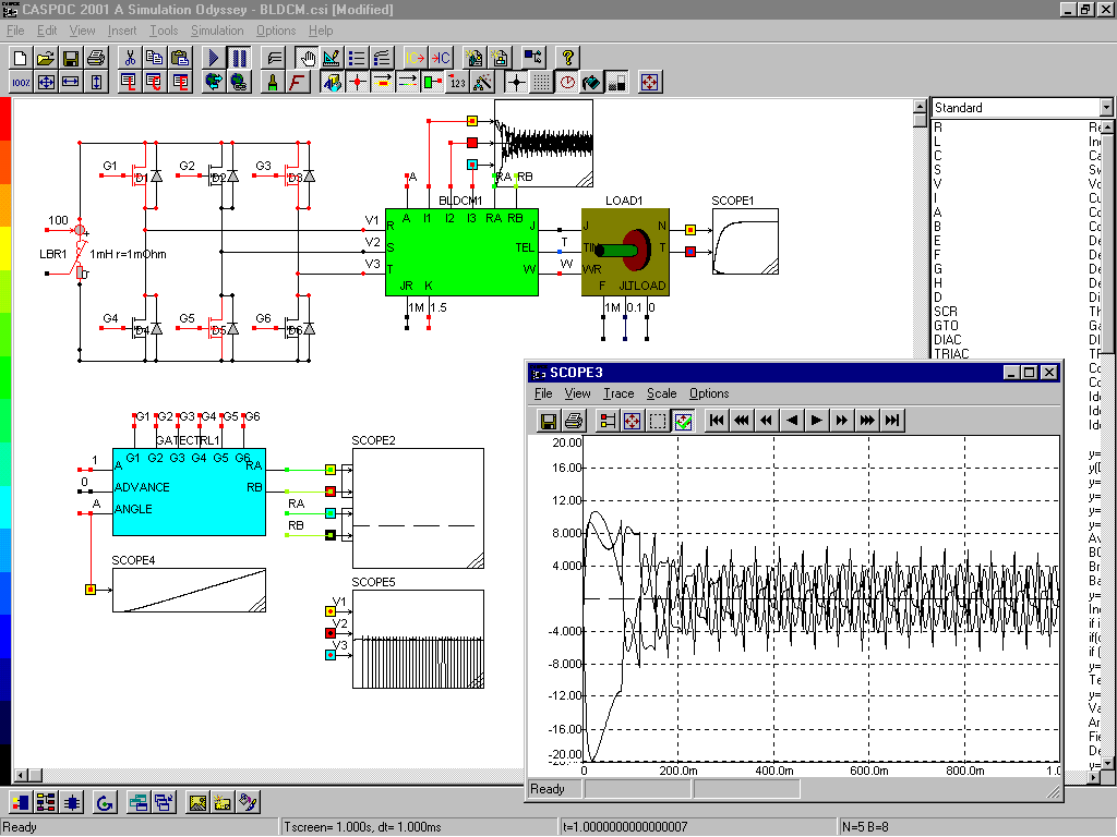
Figure 8: Brushless DC machine with 6-pulse control.
At the bottom the parameters for the brushless machine are defined, being the back-emf constant K and the inertia of the rotor. Other parameters for the machine are fixed inside the block, so the example runs also under the, in nodes limited, freeware version of Caspoc. At the top the angle of the rotor is exported, which is required for a simple control of the IGBT's. The node A indicates the angle of the rotor in radians and is connected to the left side of the block GATECTRL, which fires the IGBT's as function of the angle A. In scope 3 the currents during start-up are shown.
14.Conclusions
Animation gives valuable information about the simulation of Power Electronics and Electrical Drives. Displaying current-paths gives insight in the behavior of the circuit and can reveal failure modes. It reveals more insight in the circuit operation then only displaying simulation results in graphs. If animation is based on simulation, also complex circuits can be animated. This makes animation a practical tool for designing power electronics and electrical drives.
For power electronic circuits the values of nodal voltages and branch currents can be visualized during the simulation and the conducting semiconductors can be identified. The different modes of operation can be identified and the animation gives an overview of current distribution among the switches.
The example of the Vienna-Rectifier shows that complex current paths can be visualized to gain a better understanding of the operation of the rectifier.
For electrical drives, the moving or rotating objects can be visualized. In the case of a SRM, the dependency of the inductance on the rotor position can be displayed, giving insight in the correctness of the functioning of the model. The example of the crane with DC machine visualizes the operation of a total system, where the control of such systems can be displayed. If the machine would not stop at the desired length of the crane cable, this is clearly visible in the animation.
Animation is not a toy, it can give valuable information to the designer not only on how his design is operating but can also show the fault conditions arising during the normal operation.
15.References
Ho C-W, Ruehli A.E., Brennan P.A., The modified nodal approach to network analysis, IEEE Transactions on Circuits and Systems, Vol CAS-22, No 6, pp. 504-509, june 1975.
Schwarz A.F., Computer-aided design of microelectronic circuits and systems, Vol 1, Academic press 1987.
Franz G.A., Multilevel simulation tools for power converters, IEEE APEC CH2853-0/90/0000-0629, 1990.
Duijsen P.J. van, Multilevel modeling and simulation of power electronic converters and drive systems, Proceedings Power Conversion and Intelligent Motion (PCIM), 1994.
Kolar J.W., and Zach, F.C., A Novel Three-Phase Three-Switch Three-Level PWM Rectifier. Proceedings of the 28th Power Conversion Conference, Nuremberg, June 28-30, pp. 125-138 (1994).
Simulation Research, Caspoc 2001; A simulation Odyssey, www.caspoc.com , 2001
ANIMATION IMPROVE HIGHWAY CODE RULES LEARNING IN DEAF CANDIDATES
ANIMATION OF POWER ELECTRONICS AND ELECTRICAL DRIVES PETER J
ANIMATION OF TCE MOVEMENT AT WOBURN MASSACHUSETTS E SCOTT
Tags: animation of, animation. animation, animation, electrical, drives, power, electronics, peter
- CEL107 ANNEXE IANNEX I PAGE 6 CEL107 ANNEXE IANNEX
- CURRICULUM VITAE INFORMACION PERSONAL TOMAS ROGELIO ALARCON VASQUEZ DNI
- izjava_o_dostavi_bjanko_zaduznice_-_pravne_osobe
- CIJENJENI KORISNICI OBAVJEŠTAVAMO VAS DA PISANI PRIGOVOR NA KVALITETU
- MENU ESCOLAR DIETA SENSE GLUTEN OCTUBRE 2018 1
- FLAPJACK FUNDRAISER CHARITY GUIDE AT APPLEBEE’S BEING PART OF
- 24° GRAN PRIX REGIONALE CAMPANIATLETICA – ANNO 2019 IL
- 456001 §45600—SEMIANNUAL COMPILATION 456001 SUBPART F — AGENCY REPORTS
- TIPOS DE TEXTO LAS TIPOLOGÍAS TEXTUALES SON MÉTODOS
- REFERÊNCIA BIG ISSUES IN MOBILE LEARNING EVALUATING
- POLÍGONO DE WIKIPEDIA LA ENCICLOPEDIA LIBRE UN POLÍGONO
- ÁREA DE FOMENTO Y EMPLEO DEL 16 DE SEPTIEMBRE
- 197 DRY YOUR TEARS AFRICA BERNARD DADIE DRY YOUR
- BIBLIOGRAFÍA DEL TEMARIO 1 ALFAROLEFEVRE R APLICACIÓN DEL PROCESO
- PRISCILA SERRANO LARA SINESTESIA INTRODUCCIÓN TODOS CONOCEMOS LA PALABRA
- REALISING THE POTENTIAL OF GB RAIL FINAL INDEPENDENT REPORT
- MANUAL DE PROCEDIMIENTOS PARA LA PRECERTIFICACIÓN Y EMISIÓN DE
- 7 PARTICIPACIÓN DE ACTORES SOCIALES EN LAS OEASERE ACTIVIDADES
- PE8720 RS232 PIN CONFIGURATION DB 9 MINI DIN
- DISSECTION AND MICROSCOPY OF PLANT VASCULAR TISSUE LEARNING OUTCOMES
- MOSQUITO RECORDING SCHEME DATA FORM PLEASE COMPLETE THE
- MEDELLÍN OCTUBRE 26 DE 2020 SEÑORES MINCIENCIAS AV CALLE
- MOCIÓ PER A UN DESENVOLUPAMENT RURAL SOSTENIBLE INTEGRAL I
- 7ENTREVISTA MODELO PARA CONTADORES 1 NOMBRE 2 PROFESIÓN 3
- JAMONES EL CASTELLAR JAELKA JANVIER 2012 1 JAMÓN
- ABGEORDNETENHAUS BERLIN – 15 WAHLPERIODE DRUCKSACHE 15 1422 G
- LAKE MISSAUKEE COUNTY PARK RATES AND FEES FOR 2021
- STV 4444 EUROPEISK REGIONALISME OG MULTILEVEL GOVERNANCE FORELESINGSPLAN OG
- 0 0 WORKS SAMPLE BIDDING DOCUMENTS UNDER JAPANESE ODA
- SAVING SALVATION THE AMAZING EVOLUTION OF GRACE BY STEPHEN
 N PRESSMEDDELANDE 8E DECEMBER 2017 SG GROUP STÄLLER
 GEGRILDE KALFSENTECOTE MET KNOFLOOKJUS INGREDIENTEN 4 PERS 6
ASCCC RESOLUTION PROCEDURES SCRIPT FALL 2011 1 I
 TEL 93 540 40 24– FAX 93 540 03
 MULTICLUSTERSECTOR INITIAL & RAPID ASSESSMENT (MIRA) COMMUNITY LEVEL ASSESSMENT
 NBTF 3182010 SVEN LJUNG HUVUDENTREPRENÖRERS ANSVAR – SOLIDARANSVAR INLEDNING
 051030-death_penalty
 AYUNTAMIENTO DE ALCOBENDAS DECLARACIÓN DE DATOS BÁSICOS PARA SOLICITUD
FELNŐTTOKTATÁS OSZTÁLYKÖZÖSSÉGÉPÍTÉS (OSZTÁLYFŐNÖKI PROGRAM) ISKOLARENDSZERŰ FELNŐTTOKTATÁS 14 ÉVFOLYAM AZ
CURRICULUM VITAE DATOS PERSONALES NOMBRE Y APELLIDO CLAUDIA
COMMUNIQUÉ DE PRESSE RELATIF À L’ORGANISATION D’ASSISES NATIONALES POUR
 LA LETTRE DE MOTIVATION VOTRE PROJET ABOUTI VOUS ALLEZ
OSOBNÍ ÚČET – VÝŇATEK ZÁKLADNÍCH SAZEB PLATÍ OD 142010
 T OBS! VIKTIGT ATT DU ANGER HELA DITT PERSONNUMMER!
NA OSNOVU ČLANA 110 STAV (1) ZAKONA O IGRAMA
 NEWS RELEASE FOR IMMEDIATE RELEASE MARCH 30 2016 CONTACT
 PASAN A DOMINIO PÚBLICO EN 2020 LA BNE DIGITALIZA
 12 SUNKEL GUILLERMO UNA MIRADA OTRA LA CULTURA DESDE
 Hr212 dd Faculty Department Performance Consistency Review Report
CPM 20092 ANEXO 2 PROYECTO DE APÉNDICE DE LA
