EXERCISE 2 GEOLOGIC STRUCTURES GEOLOGY LAB 111 NAME
2006SOM3TFEP002A AGENDA ITEM 3 APEC PANDEMIC RESPONSE EXERCISECARDS EXERCISE FACILITATOR GUIDANCE LEARNING OUTCOME TO GAIN
RECONCILE AND APPROVE PCARD TRANSACTIONS EXERCISES IN THIS
0 20120814 EXERCISES ZEMAX 3 ABERRATIONS 3 PROPERTIES OF
10 THE HÜCKEL APPROXIMATION IN THIS EXERCISE YOU WILL
109 JOURNAL OF EXERCISE PHYSIOLOGYONLINE AUGUST 2021 VOLUME 24
Exercise 2: Geologic Structures
Exercise 2: Geologic Structures
Geology Lab 111 Name______________________________________________________
Objectives:
Learn what causes rock to deform or break
Learn the names of basic geologic structures
Learn how to visualize geologic structures in 3-D
Learn about the brittle-ductile transition in the crust
Why Rocks Break or Deform
Rocks break or deform under stress. Stress, technically speaking, is a force applied over a given area. Pressure and stress are actually the same thing. Your hand pressing down on the table is exerting stress (or pressure) on the table (and the table pushes back and deforms your hand!). The change in shape an object under stress experiences is called strain.
1) Think about chewing gum. Under what conditions could you make it more difficult to stretch or squish? What makes it softer? What causes it to break?
2) Now, think about rocks in relation to chewing gum. Obviously, rocks are harder, but under what conditions would they soften? Why would they break?
3) Generalize what you have thought about in relation to the strength of rocks (or of any solid). What variables (conditions) control whether they are soft or hard or if they would break?
4) Draw pictures in the space below of a solid cube being deformed. Use arrows to show the stress that is being exerted on the cube to make it deform.
5) What are real geological examples of breaks occurring in rocks?
6) How would you apply the terms plastic and brittle to what you learned above?
8) Now, go back to question 3. The general conditions, or variables, that cause solids to break or deform change with depth in the Earth. Draw a simple picture that illustrates how those conditions change from the surface down into the Earth.
9) In the drawing you just made, draw a line that separates where rocks break from where rocks deform. What geologic structures would not be found below this line?
Names of Basic Geologic Structures
For this section, you are going to make very simple drawings of real structures. Use the computers or a text book to look up the following: normal fault, reverse fault, strike-slip fault, detachment fault, anticline, and syncline. You need to label each of your drawings with the name of the type of geologic structure for your own reference. I recommend that you draw just a 2-D view of every geologic structure shown at this point. Use the boxes below for each of your drawings. In each drawing, show fat arrows indicating the direction of stress that created the structure you are drawing and write the name of the stress in the box.

3-D Views of Geologic Structures
In the space below, draw examples of a normal fault, reverse fault, strike-slip fault, and anticline/syncline pair in 3-D. You should show what the land on the surface might be like over these structures, showing the mountains, hills, and valleys in relation to the structures underneath. You also need to draw arrows showing the stress that created these structures. There are no boxes provided because you might want lots of space for your drawings.
The Brittle-Ductile Transition in the Crust
Read the following article and answer the questions that follow.
The
Evolution of the Seismic-Aseismic Transition during the
Earthquake
Cycle: Constraints from the Time-Dependent Depth
Distribution
of Aftershocks
Frédérique Rolandone, Roland Bürgmann and Robert Nadeau
Introduction
We have demonstrated that aftershock distributions after several large earthquakes show an immediate deepening from pre-earthquake levels, followed by a time-dependent postseismic shallowing (Rolandone et al., 2002). We use these seismic data to constrain the depth variations with time of the seismic-aseismic transition throughout the earthquake cycle. Most studies of the seismic-aseismic transition have focussed on the effect of temperature and/or rock composition and have shown that the maximum depth of seismic activity is well correlated with the spatial variations of these two parameters. However, little has been done to examine how the maximum depth of seismogenic faulting varies locally, at the scale of a fault segment, with time during the earthquake cycle.
The mechanical behavior of rocks in the crust is governed by frictional behavior and at greater depth by plastic flow. The coupling between the brittle and ductile layers and the depth extent and behavior of the transition zone between these two regimes is a fundamental question. Mechanical models of long-term deformation (Rolandone and Jaupart, 2002) suggest that the brittle-ductile transition is a wide zone where deformation is caused both by slip and ductile flow. Geologic observations (Sibson, 1986; Scholz, 1990; Trepmann and Stockhert, 2002) indicate that the depth of the seismic-aseismic transition varies with strain rate and therefore is also expected to change with time throughout the earthquake cycle. The maximum depth of seismogenic faulting is interpreted either as the transition from brittle faulting to plastic flow in the continental crust, or as the transition in the frictional sliding process from unstable to stable sliding. The seismic-aseismic transition therefore reflects a fault zone rheology transition or a more distributed transition from brittle to ductile deformation mechanisms.
Results
We investigate the time-dependent depth distribution of aftershocks in the Mojave Desert. We apply the double difference method of Waldhauser and Ellsworth (2000) to the region of the M 7.3 1992 Landers earthquake to relocate earthquakes. Time-dependent depth patterns of seismicity have been identified in only few previous studies (Doser and Kanamori, 1986; Schaff et al., 2002) and never quantified. This was mainly due to the problem of the accuracy of the hypocenter locations. Accurately resolving depth is the most challenging part of earthquake location. With new relocation techniques, we can investigate the time-dependent depth distribution of seismicity to reveal more intricate details in the patterns of deformation which take place during an earthquake cycle.
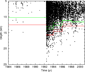
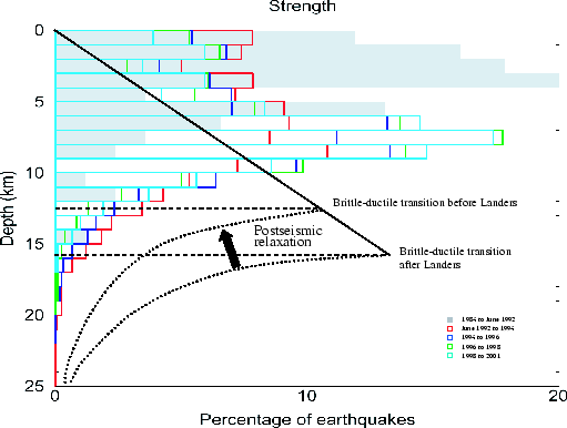
In this study, we focus on quantifying the temporal pattern of the deepest aftershocks. We calculate the d95%, the depth above which 95% of the earthquakes occur, and we also calculate the d5%, the average of the 5% of the deepest earthquakes for a constant number of events. We compare our results with the same statistics for the Hauksson relocations (catalog from Hauksson (2000) with a vertical error cutoff of 1.5 km). We specifically investigate (1) the deepening of the aftershocks relative to the background seismicity, (2) the time constant of the postseismic shallowing of the deepest earthquakes. Figure 18.1 shows the time-dependent depth distribution of seismicity for the Johnson Valley fault that ruptured in the 1992 Landers earthquake. Our analysis reveals a strong time-dependence of the depth of the deepest aftershocks. In the immediate postseismic period, the aftershocks are deeper than the background seismicity, followed by a time-dependent shallowing. Figure 18.2 shows the same data but in the form of histograms and relate them to the deepening of the brittle-ductile transition after the mainshock. The temporal variations of the depth of the brittle-ductile transition reflect the strain-rate changes at the base of the seismogenic zone.
The analysis of seismic data to resolve the time-dependent depth distribution of the seismic-aseismic transition provides additional constraints on fault zone rheology, which are independent of geodetic data. Together with geodetic measurements, these seismological observations form the basis for developing more sophisticated models for the mechanical evolution of strike-slip shear zones during the earthquake cycle.
|
Figure 18.1: Time-dependent depth distribution of seismicity for the Johnson Valley fault. The red curve shows the statistics for the d5% and the green for the d95% (see text). The dashed lines show the same statistics for the Hauksson relocations and are in very good agreement with our results. |
|
|
|
Figure 18.2: Histograms of the depth distribution of seismicity for different time periods. Overlaid is the strength of the brittle and ductile materials. |
Acknowledgements
This research is supported by the Southern California Earthquake Center and an IGPP/LLNL grant.
References
Doser, D.I., and Kanamori H., Depth of seismicity in the Imperial Valley region (1977-1983) and its relationship to heat flow, crustal structure, and the October 15, 1979, earthquake. J. Geophys. Res., 91, 675-688, 1986.
Hauksson, E., Crustal structure and seismicity distribution adjacent to the Pacific and North America plate boundary in southern California, J. Geophys. Res., 105, 13,875-13,903, 2000.
Rolandone, F., and C. Jaupart, The distribution of slip rate and ductile deformation in a strike-slip shear zone, Geophys. J. Int., 148, 179-192, 2002.
Rolandone, F., R. Bürgmann and R.M. Nadeau, Time-dependent depth distribution of aftershocks: implications for fault mechanics and crustal rheology, Seism. Res. Lett., 73, 229, 2002.
Schaff, D.P., G.H.R. Bokelmann, G.C. Beroza, F. Waldhauser and W.L. Ellsworth, High resolution image of Calaveras Fault seismicity, J. Geophys. Res., 107 (B9), 2186, doi:10.1029/2001JB000633, 2002.
Scholz, C.H., Earthquakes and friction laws Nature, 391, 37-42, 1998.
Sibson, R.H., Earthquakes and rock deformation in crustal fault zone, Ann. Rev. Earth Planet. Sci, 14, 149-175, 1986.
Trepmann, C.A., and B. Stockhert, Cataclastic deformation of garnet: a record of synseismic loading and postseismic creep, J. Struct. Geol., 24, 1845-1856, 2002.
Waldhauser, F., and W. L. Ellsworth, A double-difference earthquake location algorithm: method and application to the northern Hayward fault, California, Bull. Seismol. Soc. Am., 90, 1353-1368, 2000.
QUESTIONS ON THE ARTICLE ABOVE:
1) Look at Figure 18.1. Explain what happened in 1992 that caused the change in seismicity in this area.
2) What is the depth range of the earthquake foci shown in Figure 18.1?
3) At what depth to earthquakes cease before 1992? At what depth do they cease after 1992? What is the meaning of this depth at which earthquakes cease? What is this depth called?
4) How did the event in 1992 change the depth distribution of the earthquake foci? Refer to figure 18.2.
5) How do the authors interpret this change in the depth distribution? Explain what they think this shows about the brittle-ductile transition in the crust.
11 TRANSFORMATION EXERCISES COMPLETE THE SECOND SENTENCE OF
150 JOURNAL OF EXERCISE PHYSIOLOGYONLINE APRIL 2018 VOLUME 21
150080 INTRODUCTION TO INFORMATION SYSTEMS HMTL INCLASS LAB EXERCISE
Tags: exercise 2:, exercise, geologic, geology, structures
- 2018 DESERT VISTA HIGH SCHOOL SADIES DANCE SATURDAY FEBRUARY
- COMPANY NAME REGISTER OF LEGAL AND OTHER REQUIREMENTS DOCUMENT
- NEDOVOLJENO OGLAŠEVANJE PODROBNEJŠI OPIS KAZALO 10 NEDOVOLJENO OGLAŠEVANJE 3
- 49 ROČNÍK FYZIKÁLNEJ OLYMPIÁDY V ŠKOLSKOM ROKU 200708 ZADANIA
- POLITECHNIKA WROCŁAWSKA WYDZIAŁ CHEMICZNY ZAKŁAD MATERIAŁÓW POLIMEROWYCH I WĘGLOWYCH
- 4 LA MÚSICA INSTRUMENTAL EN EL RENACIMIENTO INTRODUCCIÓN DEL
- ANNEX NÚM 9 REPORTATGE FOTOGRÀFIC RECONSTRUCCIÓ TRIDIMENSIONAL DEL CREUER
- MINISTERIO DE DESARROLLO RURAL Y TIERRA MINISTERIO DE DESARROLLO
- TEMARIO GENERAL DE LA ESTT OEP 2011 ESPECIALIDAD RÉGIMEN JURÍDICO DEL TRÁFICO ELABORADO EN 2011
- COMUNIDAD ANDINA SECRETARIA GENERAL RESOLUCIÓN 111 6 DE AGOSTO
- SEKTOR PRAVNIH OPĆIH I POSLOVA USKLAĐENOSTI DIREKCIJA NABAVE I
- SPECIALISTSJUKSKÖTERSKEUTBILDNING INRIKTNING PSYKIATRISK VÅRD 60 HP LITTERATURLISTA GÄLLER FROM
- 20120406 BRFEKHOLMENHOTMAILCOM EKHBLADET ÅRGÅNG 2012 NR1(JANMARS) ÄNTLIGEN
- APRIL 10TH 2014 H E U JOY OGWU PERMANENT
- QUALITY ASSURANCE PLAN CHECKLIST GUIDELINES FOR THE QUALITY ASSURANCE
- VÁŽENÝ PANE POLÁK OPIS TŘÍ VĚT Z VAŠEHO DOPISU
- FRÅGA TILL STATSRÅD 20130213 TILL LANDSBYGDSMINISTER ESKIL ERLANDSSON (C)
- UNIVERSITÀ DEGLI STUDI “LA SAPIENZA” ROMA FACOLTÀ DI LETTERE
- „W WYCHOWANIU CHODZI WŁAŚNIE O TO AŻEBY CZŁOWIEK STAWAŁ
- 20090731 KLUBB 119 FACKET INFORMERAR INFORMATION OM VAD SOM
- APUNTES CONECTORES TEXTUALES ES IMPORTANTE QUE OS FAMILIARICÉIS CON
- TC ZİRAAT BANKASI AŞ VE THALK BANKASI AŞ MENSUPLARI
- ASIAN JOURNAL OF SOCIAL SCIENCE AND MANAGEMENT TECHNOLOGY ISSN
- INTRODUCCIÓN EL OBJETIVO DE ESTE MATERIAL ES ENSEÑAR A
- DALARNAS BORDTENNISFÖRBUND BJUDER IN TILL REGION TOP 12 DATUM
- WEEKLY SITREP A&E – DEFINITION AND GUIDANCE WEEKLY TRUST
- TC SİVAS CUMHURİYET ÜNİVERSİTESİ YILDIZELİ MESLEK YÜKSEKOKULU MÜDÜRLÜĞÜ MESLEK
- ACTA DE CONFORMACIÓN DE VEEDURÍA CIUDADANA EN EL MUNICIPIO
- 2011 SLOGAN CONTEST HELP CLEAN AIR PARTNERS SPREAD THE
- UNIVERZITET U SARAJEVU ŠUMARSKI FAKULTET NASTAVNI PLAN I PROGRAM
ANSØGNING OM STØTTE FRA N STORRS KONTO UNDER DIABETESFORENINGENS
ASTROLABIO REVISTA ELECTRÓNICA DE FILOSOFÍA AÑO 2005 NÚM 1
 AUSZEICHNUNG DER HISTORISCHE GASTBETRIEB DES JAHRES IN SÜDTIROL KRITERIEN
 PIELIKUMS NR2 IEPIRKUMA IDENTIFIKĀCIJAS NR APES ND 20154 PRETENDENTA
28GÜVENLİK YENİLEME SINAV SORU VE CEVAPLARI 1) İNSAN HAKLARINI
BARRY LOEWER CURRICULUM VITAE (SPRING 2010) CONTACT INFORMATION DEPARTMENT
 KENTUCKY AND APPALACHIA PUBLIC HEALTH TRAINING CENTER STRATEGIC PLANNING
 ICES CM 2019E326 IDENTIFICATION OF CROSS BOUNDARY MANAGEMENT UNITS
 BSD GEMS 050 DELEGATES POLICIES DELEGATES USED TO COMPLETE
RESIDENT FOOD PREFERENCES THERAPEUTIC DIETS RESIDENT NAME DATE OF
 DATUM…………………… BLANKETT FÖR SAMMANSTÄLLNING AV SYNPUNKTERKLAGOMÅL AVDELNINGENHET …………………………………………………………
TOKAT GAZIOSMANPAŞA ÜNIVERSITESI GIZLILIK SÖZLEŞMESI TOKAT GAZİOSMANPAŞA ÜNİVERSİTESİ GİZLİLİK
 IZHODIŠČA ZA OPPN CESTA NA GRADEC EUP MIR145 GI
BIJLAGE 1 BIJLAGE BIJ ARTIKEL … CONTROLEPROTOCOL CONTROLEVERKLARING SUBSIDIEREGELING
 REQUISITOS QUE DEBEN CUMPLIR LOS GRADUADOS QUE SE PRESENTAN
VÄXJÖ UNIVERSITET HID 180 INSTITUTIONEN FÖR HUMANIORA MAGISTERUPPSATS HISTORIA
 QUÍMICA TAREA 43 ENERGÍA Y CINÉTICA QUÍMICA LA CUEVA
CULTURA E INTEGRACIÓN CULTURA E INTEGRACIÓN HELIO VERA INTRODUCCIÓN
AYUNTAMIENTO DE FRESNO DE CARACENA PLIEGO DE CONDICIONES ECONÓMICOADMINISTRATIVAS
ADMISSIONS ARRANGEMENTS FOR HARRIS INVICTUS ACADEMY CROYDON 202021 ADMISSION
