LECTURE 11—INFILTRATION SOME OF THE RAIN THAT FALLS EVAPORATES
111 DERIVING DYNAMIC PROGRAMMING ADVANCED MATH THIS LECTURE REALLY13 ALLAN MACRAE JEREMIAH LECTURE 2 © 2013 DR
13 FRIDAY ALL NIGHT SERVICE TITLE LECTURE ON GENESIS
2 ECON4925 LECTURE PLAN LECTURE PLAN ECON4925 2006 (REV1)
2 LECTURE USE OF COHERENCE OF LASER LIGHT PHOTON
20 ALL OF LIFE IS A PROJECTION LECTURE BY
Lecture 11—Infiltration
Some of the rain that falls evaporates back into the atmosphere,
and some of it hits the ground.
How do we find out how much of it sinks in, and how much of it
runs off?
This part of the hydrologic cycle provides the critical link
Intuitively, we can talk about what should happen, and we can even write an equation that mimics what we said intuitively, but bear in mind that
the process our model says should be happening probably doesn’t.
Is rain more likely to sink into sand, or into clay? Some material
properties of the ground affect how fast rain can sink in. The material
property in this case is permeability, and it’s a function not only of
how many void spaces there are in a soil, but also how connected
they are and how large they are.
Typically permeability is determined empirically. If a soil has high permeability, more water will sink in, and low permeability means more runoff.
Many of the “connected spaces” are fairly fragile, and one problem is that the impact energy of raindrops can destroy that shallow structure. This decreases the surface area available for infiltration.
Water actually attaches itself in a thin layer around every grain in the
soil, so that the size of the void spaces actually shrinks as the soil
gets wetted. Clearly, then, there will be some time dependence on
how much water sinks in vs. runs off.
Horton (1940) came up with an equation that satisfies our intuitive
notions about how all this should work. Here’s the equation:
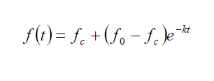
where f is the infiltration capacity (in in/hr),
f0 is the initial infiltrationcapacity,
fc is the final infiltration capacity,
and k is an empirical constant that says something about how long it takes for rain to force the soil from its initial to its final infiltration capacity.
This has since been experimentally shown to be an effective gauge of infiltration.
Example: The initial infiltration capacity of a watershed is estimated as 1.5 in/hr, and the time constant taken to be 0.35 hr -1. The equilibrium capacity is estimated as 0.2 in/hr.
(a) What are the values of f at t = 10 min, 30 min, 1 hr, 2 hr, and 6 hr, and
(b) what is the total volume of infiltration over the 6 hour time period?
From the Horton equation, we have:
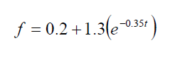
(a) Substituting in values of t yields:
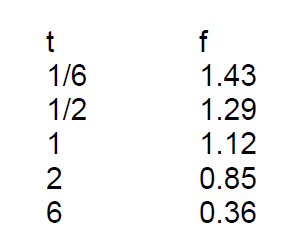
(b) The table on the previous page, when plotted, looks like the graph here.
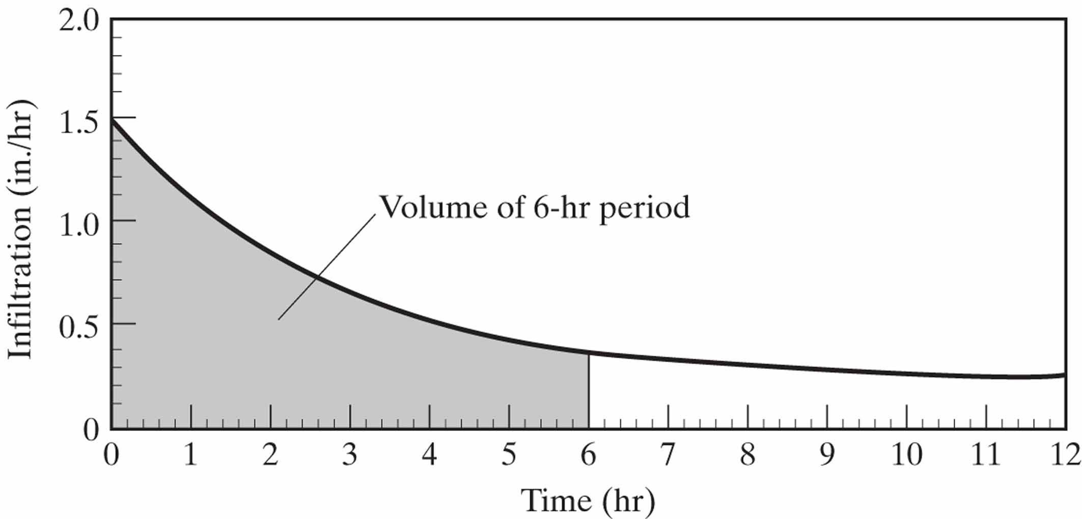
The volume of water can be found by taking the definite integral
(use font SymbolMT ∫) under the curve from 0 to 6 hours. Here the integration is easy, and turns out like this:
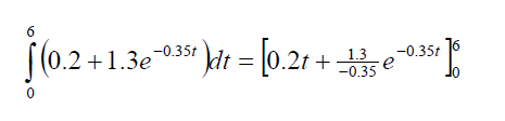
Evaluating the right side for t = 6 and then subtracting the values for t=0 yields an answer of 4.46 inches over the watershed.
The Horton equation assumes that rainfall exceeds infiltration rate, so that there must be ponding at the surface and reduction in infiltration rate with time. If, however, the rainfall intensity doesn’t exceed the rainfall rate, there’s no need to drop the infiltration rate.
As a result, some researchers have suggested that infiltration capacity should vary with the cumulative infiltration volume and not with time. Unfortunately, this requires iteration between the equation for cumulative infiltration volume (which we got in the example) and the Horton equation. As a result this technique is mostly used in computer simulation.
Part 2: Phi
The simplest way of measuring infiltration is purely empirical. We could
simply assume that infiltration is constant during the whole rainfall
period, and find a constant (call it φ) that relates how much water ran
off for a given rainfall. The constant would be useable to estimate
runoff for future events.
Here’s an example:
Use the rainfall data listed to determine the φ index for a watershed
h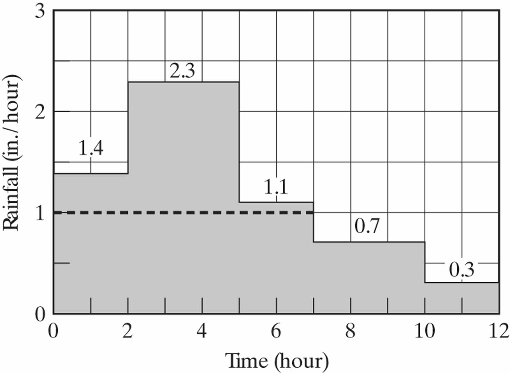 aving
a total runoff of 4.9 inches for this storm.
aving
a total runoff of 4.9 inches for this storm.
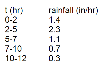
The first step is to make a hyetograph from the data, as shown in the
graph.
All we need after that is to find the line level that allows the
“runoff” part of the hyetograph to be equal to exactly 4.9 inches.
![]()
You can either solve this equation directly, or go ahead and find φ by
trial and error. In this case, assuming φ = 1.5 in/hr yields 2.4 inches
of runoff, which is too low; assuming φ = 0.5 in/hr yields 9.0 inches of
runoff, which is too high. The answer for this is φ = 1.0 in/hr.
2002 FRESHFIELDS LECTURE 19 ARB INT’L 279 (2003) ARBITRATION’S
3 TEST QUESTIONS – BIT LECTURE 1 OBJECTIVES AND
3012 FUNDAMENTALS OF MATERIALS SCIENCE FALL 2003 LECTURE 10
Tags: 11—infiltration some, evaporates, falls, lecture, 11—infiltration
- ANNEXURE 7 – A 27 SECTION 7 STEEL
- REGULAMIN ZARZĄDU POLSKIEJ FEDERACJI SCRABBLE § 1 ZADANIA I
- THE VALUES OF INCLUSION EVERYONE IS BORN IN WE
- STANDARD MODEL LHC APRIL 8TH – 11TH 2014 MADRID
- SURVEY RETEST S IGNATURE TITLE PHONE DATE FIELD NAME
- GDCA VETERINARIAN MAP LIST ALASKA GOLDEN HEART VETERINARY SERVICES
- D OLPHIN COAST WIRELESS PO BOX 713 BALLITO 713
- NAÇÃO E IDENTIDADE NACIONAL NO LIVRO DIDÁTICO DE HISTÓRIA
- HRVATSKA AKADEMSKA I ISTRAŽIVAČKA MREŽA – CARNET CDA 0038
- DRUŠTVO NOVINARJEV SLOVENIJE OKROGLA MIZA PASTI MEDIJSKE REGULACIJE IN
- …………………………………………… LİMİTED ŞİRKETİ … … TARIHINDE YAPILAN OLAĞANÜSTÜ
- MATURA 2015 LISTA TEMATÓW NA USTNĄ CZĘŚĆ EGZAMINU MATURALNEGO
- MẪU DANH SÁCH PHƯƠNG TIỆN VẬN CHUYỂN NGƯỜI ĐIỀU
- COMPTE RENDU DE TP PURIFICATION ET STABILITE DE LA
- METODY SPEKTROSKOPOWE W ANALIZIE CHEMICZNEJ ĆW 3 SYMULACJA WIDM
- SUPPORT STAFF PLEASE STATE WHICH ARK ACADEMY YOU HAVE
- EMERGENCY OPERATIONS PLAN 2009 1 INTRODUCTION PAGE NO
- LA CASA MALDITA H P LOVECRAFT RARA VEZ
- 28 SVERIGES GRODOR OCH PADDOR © SIMON KÄRVEMO
- INSTALACIONES TÉRMICAS EN LOS EDIFICIOS CERTIFICADO DE 1ª INSPECCIÓN
- CASE TITLE [WELL NOTIFICATION TITLE] REFERENCE NUMBER
- 27 NO7762 LEY GENERAL DE CONCESIÓN DE OBRAS PÚBLICAS
- 33 FEDERAAL AGENTSCHAP VOOR DE VEILIGHEID VAN DE VOEDSELKETEN
- ZAŁĄCZNIK NR 2 DO USTAWY Z DNIA 30 MAJA
- EXTRA DEUTSCH 3 SAM HAT EIN DATE ÜBUNGEN ÜBUNG
- XI USING A SPECTROPHOTOMETER BACKGROUND A SPECTROPHOTOMETER IS PRIMARILY
- D OLPHIN SPLASH CENTENNIAL LANE ELEMENTARY SCHOOL PTA HTTPWWWCLESPTAORG
- FINAL DRAFT ENERGY STAR® SPECIFICATION FOR RESIDENTIAL CEILING FANS
- PROF ELIZABETH MADDOCK DILLON ENGLISH G213 THREE REVOLUTIONS IN
- Tillståndsansökan för Arrangemang av Internationell Tävling med Svenska lag
 DEPARTAMENTO DE EDUCACIÓN FÍSICA E DEPORTIVA ACTA DE CUALIFICACIÓN
 O MENTIREIRO VERDADEIRO PRIMEIRO DÍA QUE É O QUE
 BEOBACHTUNGSBOGEN AUFSCHLAG VON UNTEN VORSCHLAG ZUR DURCHFÜHRUNG A SCHLÄGT
 DIALPLANCONFIGURATION EXTENSION NAMES AND PATTERNS EXTENSION NAMES
 33 TELEIMMERSION SEMINAR REPORT ‘03 INTRODUCTION IT IS 2010
 SEMESTER CHANGE AN ADMISSION APPLICATION IS ELIGIBLE FOR SEMESTER
 UBND HUYỆN QUỐC OAI CỘNG HÒA XÃ HỘI CHỦ
 TOXINA BOTULÍNICA TIPO A CFYT HU VIRGEN DEL ROCÍO
 ACUERDO 22021 DE 7 DE ENERO DE LA JUNTA
CREATIVE THINKING THEORY TECHNIQUES AND ASSESSMENT CREATIVE THINKING (A
 LICEO MIGUEL RAFAEL PRADO GUÍA DE DEBATE 3 JUNIO
 DIU CHIRURGIE ET ANESTHÉSIE AMBULATOIRE 20142015 CHRU TROUSSEAU
THE NATIONAL INFORMATION CLEARINGHOUSE ON CHILDREN WHO ARE DEAFBLIND
TITLE AS IT WAS IN THE DAYS OF JEREMIAH
 SPOROČILO ZA JAVNOST ŠT 150816 STRANI 3 ŽIVAHNA TURISTIČNA
NORMAS BRASILEIRAS DE CONTABILIDADE NBC TA 220 – CONTROLE
 FORMATO VERSIÓN 01 ENTREGABLE DE PROYECTOS DE AULA 3
 A TURCARA DAN KANDUNGAN MODUL BENGKEL PERUNDANGAN CUKAI BARANG
DA 12523 RELEASED APRIL 2 2012 COMMISSION SEEKS COMMENT
 MEDIDAS DE LONGITUD 1 ¿CUÁNTOS METROS SON? 3 HM
